LET US TAKE A LOOK AT HOUSE PRICE AND EMPLOYMENT TRENDS.
House prices in the Unitest States have been increasing at a rapid pace, about 7 percent on an annual basis. How does that relate to employment growth? And how do those trends vary by geography. Let’s take a look.
Per usual, I will post R code and you can follow along.
Data
Following recent posts (see here and here for example), we will use the Freddie Mac House Price Index an Excel spreadsheet can be downloaded here.
We’ll get employment data from the U.S. Bureau of Labor Statistics via FRED. See here for more on using the quantmod and tidyquant packages to work with FRED data.
The following code will wrangle our data (out of the spreadsheet and out of FRED).
###############################################################################
#### Load libraries
###############################################################################
library(tidyverse)
library(data.table)
library(tibbletime)
library(tidyquant)
library(magrittr)
library(viridis)
library(scales)
library(readxl)
library(geofacet)
library(cowplot)

###############################################################################
#### Load state data (download spreadsheet in a data directory)
###############################################################################
df<-read_excel("data/states.xls",
               sheet = "State Indices",
               range="B6:BB522" )

# make dates
df$date<-seq.Date(as.Date("1975-01-01"),as.Date("2017-12-01"),by="1 month")
df.state<-df %>% gather(geo,hpi,-date) %>% mutate(type="state",state=geo)

df.state<-
  df.state %>% group_by(geo) %>% mutate(hpa=hpi/shift(hpi,12)-1,
                                        hpa1=hpi/shift(hpi,1)-1,
                                        hpilag12=shift(hpi,12,fill=NA),
                                        hpimax12=rollmax(hpi,13,align="right",fill=NA),
                                        hpimin12=-rollmax(-hpi,13,align="right",fill=NA)) %>% ungroup()

df.state<-df.state %>% group_by(date) %>%
  mutate(us.hpa=hpa[geo=="United States not seasonally adjusted"],
         us.hpi=hpi[geo=="United States not seasonally adjusted"]) %>%
  mutate(up=ifelse(hpa>us.hpa,hpa,us.hpa),
         down=ifelse(hpa<=us.hpa,hpa,us.hpa),
         dlabel=paste(as.character(date,format="%B-%Y")," \n ")
  ) %>%
  ungroup()

df.state <- filter(df.state,
                   !( state %in% c("United States not seasonally adjusted","United States seasonally adjusted")))
dlist<-unique(filter(df.state,year(date)>1999)$date)
df.state<- df.state %>% group_by(state) %>% mutate(id = row_number()) %>% ungroup()

# get hpa by state and year (December only)
df.state %>% mutate(year=year(date)) %>% filter(month(date)==12 & year>1989) %>% select(year,state,hpa) -> df.state2

#####################################################################################
## Step 2: go get data from FRED ##
#####################################################################################

tickers<-c(paste0(us_state_grid2$code,"NA"),      # nonfarm employment is NA (monthly, SA)
           paste0(us_state_grid2$code,"POP"),     # resident population (annual)
           paste0(us_state_grid2$code,"BPPRIV")  # private building permits (monthly, NSA)
           )

df<-tq_get(tickers,get="economic.data",from="1990-01-01")

#####################################################################################
## Organize the data ##
#####################################################################################
df<-mutate(df,
           state = substr(symbol,1,2),
           var   = substr(symbol,3,10))
# get population by year

df %>% filter(var=="POP") %>% mutate(year=year(date)) %>% group_by(state,year) %>% summarize(POP=sum(price)) -> df.pop
df %>% filter(var=="BPPRIV") %>% mutate(year=year(date)) %>% group_by(state,year) %>% summarize(PERMITS=sum(price)) -> df.permits
df %>% filter(var=="NA" & month(date)==12) %>% mutate(year=year(date)) %>% group_by(state,year) %>% summarize(EMP=sum(price)) -> df.emp
df3 <- merge(df.emp,
             df.pop,
             by=c("state","year")) %>% merge(df.permits, by=c("state","year"))
df3 %<>% group_by(state) %>% mutate(perm2pop=PERMITS/POP, EMPg=Delt(EMP,k=1), POPg=Delt(POP,k=1), PERMg=Delt(PERMITS,k=1), eg2permg=EMPg/PERMg) %>% ungroup()
df4<-left_join(df.state2,df3,by=c("state","year"))

# Get national data
# employment via FRED
df.us<-tq_get("PAYEMS",get="economic.data",from="1975-01-01") %>% mutate(eg=Delt(price,k=12))

# Get US house prices
df.hpius <- filter(df.state,state=="AK") %>% select(date,us.hpa,us.hpi)

df.us<-left_join(df.us,df.hpius,by="date")
National trends
Let’s plot national trends. First with two line plots and then with a scatterplot.
g.emp<-
  ggplot(data=df.us,aes(x=date,y=eg))+geom_line()+
  geom_rect(data=recessions.df, inherit.aes=F, aes(xmin=Peak, xmax=Trough, ymin=-Inf, ymax=+Inf), fill='darkgray', alpha=0.5) +
  geom_point(data=filter(df.us,date=="2018-01-01"),color="red")+
  theme_minimal()+
  geom_hline(yintercept=0,color="black")+
  scale_y_continuous(labels=percent,sec.axis=dup_axis())+
  theme(legend.position="top",
        plot.caption=element_text(hjust=0),
        plot.subtitle=element_text(face="italic"),
        plot.title=element_text(size=16,face="bold"))+
  labs(x="",y="Percent",
       title="U.S. Nonfarm Employment Growth",
       subtitle="12-month percent change",
       caption="@lenkiefer Data Source: U.S. Bureau of Labor Statistics, shaded bars NBER Recessions.\nretrieved from FRED, Federal Reserve Bank of St. Louis; https://fred.stlouisfed.org/series/PAYEMS, February 26, 2018")

g.hpa<-
  ggplot(data=df.us,aes(x=date,y=us.hpa))+geom_line()+
  geom_rect(data=recessions.df, inherit.aes=F, aes(xmin=Peak, xmax=Trough, ymin=-Inf, ymax=+Inf), fill='darkgray', alpha=0.5) +
  geom_point(data=filter(df.us,date=="2017-12-01"),color="red")+
  theme_minimal()+
  geom_hline(yintercept=0,color="black")+
  scale_y_continuous(labels=percent,sec.axis=dup_axis())+
  theme(legend.position="top",
        plot.caption=element_text(hjust=0),
        plot.subtitle=element_text(face="italic"),
        plot.title=element_text(size=16,face="bold"))+
  labs(x="",y="Percent",
       title="U.S. House Price Growth",
       subtitle="12-month percent change",
       caption="@lenkiefer Data Source: Freddie Mac House Price Index for the United States")

g.panel<-plot_grid(g.emp,g.hpa,ncol=1)
g.panel
g.scatter<-
  ggplot(data=df.us, aes(x=eg,y=us.hpa))+geom_path(color="lightgray",alpha=0.75)+geom_point()+stat_smooth(method="lm",fill=NA,linetype=2)+
  theme_minimal()+
  geom_hline(yintercept=0,color="black")+
  geom_vline(xintercept=0,color="black")+
  scale_y_continuous(labels=percent,sec.axis=dup_axis())+
  scale_x_continuous(labels=percent,sec.axis=dup_axis())+
  theme(legend.position="top",
        plot.caption=element_text(hjust=0),
        plot.subtitle=element_text(face="italic"),
        plot.title=element_text(size=16,face="bold"))+
  labs(x="Employment growth (12-month % change)",y="House Price growth (12-month % change)",
       title="U.S. Nonfarm Employment and House Price Growth",
       subtitle="12-month percent change",
       caption="@lenkiefer Data Source: Freddie Mac House Price Index, U.S. Bureau of Labor Statistics.\nemployment data retrieved from FRED, Federal Reserve Bank of St. Louis; https://fred.stlouisfed.org/series/PAYEMS, February 26, 2018")
g.scatter
The national plot shows a reasonably strong correlation between employment growth and house prices. When employment growth is weaker, house prices tend to rise less rapidly or even fall.
State trends
Let’s look at what’s going on at the state level. First, let’s plot house price and employment trens separately using geofacets.
yy<-2017
dfq<-filter(dfq.all,year==yy)
dfb2<-filter(dfb,year==yy)

ggplot(data = dfb, aes(x=year,y=hpa,fill=hpa))+geom_col()+facet_geo(~state)+
  scale_fill_viridis(option="B",label=percent,name="12-month percent change")+
  scale_y_continuous(labels=percent)+scale_x_continuous(labels=c("'90","'00","'10","'17"), breaks=c(1990,2000,2010,2017))+
  theme(axis.text.x=element_text(size=8),legend.key.width=unit(2,"cm"),
        axis.text.y=element_text(size=8),
        legend.position="top",
        plot.caption=element_text(hjust=0),
        plot.subtitle=element_text(face="italic",hjust=0,size=14),
        plot.title=element_text(size=18,face="bold",hjust=0))+
  labs(x="",y="12-month percent change",title="House price trends by state",subtitle="y/y % change in December",caption="@lenkiefer Source: Freddie Mac House Price Index")
ggplot(data = dfb, aes(x=year,y=EMPg,fill=EMPg))+geom_col()+facet_geo(~state)+
scale_fill_viridis(option="B",label=percent,name="12-month percent change")+
scale_y_continuous(labels=percent)+scale_x_continuous(labels=c("'90","'00","'10","'17"), breaks=c(1990,2000,2010,2017))+
theme(axis.text.x=element_text(size=8),legend.key.width=unit(2,"cm"),
axis.text.y=element_text(size=8),
legend.position="top",
plot.caption=element_text(hjust=0),
plot.subtitle=element_text(face="italic",hjust=0,size=14),
plot.title=element_text(size=18,face="bold",hjust=0))+
labs(x="",y="12-month percent change",title="Employment trends by state",subtitle="y/y % change in December",caption="@lenkiefer Source: U.S. Bureau of Labor Statistics Nonfarm Payroll Emmployment (SA)")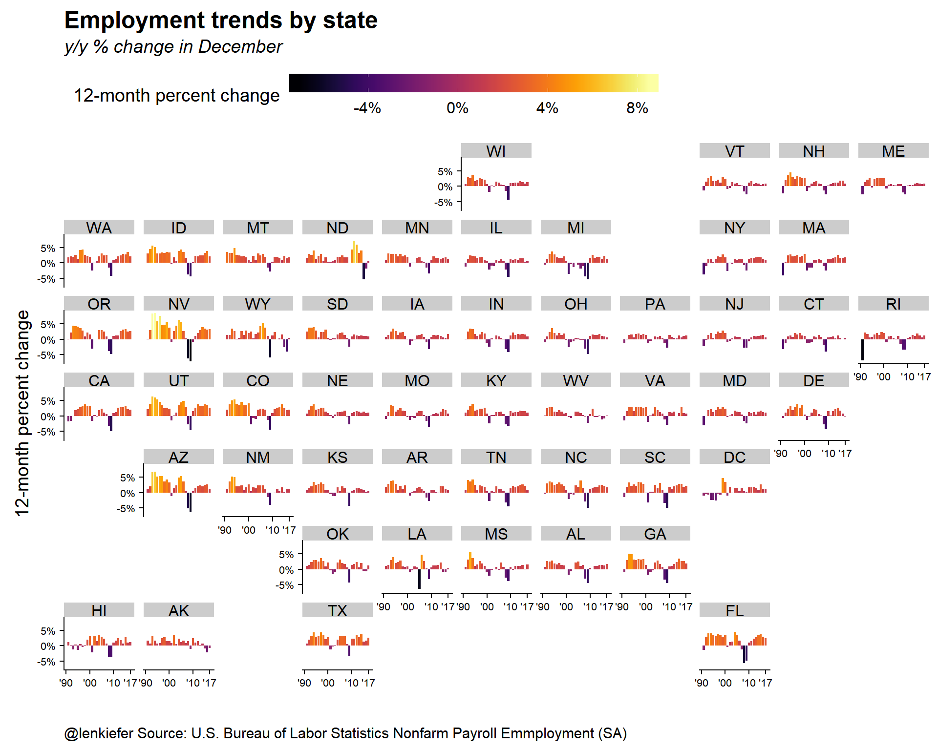 Now we can combine the employment and house price trends into a single plot. This is a bivariate tilegrid map we made last year.
First let’s make a scatter plot, and then add the tilegrid map. We will focus first on the latest available data, with year-over-year percent changes in December of 2017.
g.xy<-
  ggplot(data=dfb2,
         aes(x=EMPg,y=hpa,label=state,
             # see http://lenkiefer.com/2017/04/24/bivariate-map/
             # for explanation on the color/fill/alpha
             color=atan(y/x),
             fill=atan(y/x),
             alpha=x+y ))+

  # Shade areas based on the terciles
  geom_rect(data=dfq,aes(xmin=-Inf,xmax=x1,ymin=hpa1,ymax=hpa2,fill=atan(2/1),alpha=3/2))+
  geom_rect(data=dfq,aes(xmin=x1,xmax=x2,ymin=hpa1,ymax=hpa2,fill=atan(2/2),alpha=4/2))+
  geom_rect(data=dfq,aes(xmin=x2,xmax=Inf,ymin=hpa1,ymax=hpa2,fill=atan(2/3),alpha=5/2))+

  geom_rect(data=dfq,aes(xmin=-Inf,xmax=x1,ymin=-Inf,ymax=hpa1,fill=atan(1/1),alpha=2/2))+
  geom_rect(data=dfq,aes(xmin=x1,xmax=x2,ymin=-Inf,ymax=hpa1,fill=atan(1/2),alpha=3/2))+
  geom_rect(data=dfq,aes(xmin=x2,xmax=Inf,ymin=-Inf,ymax=hpa1,fill=atan(1/3),alpha=4/2))+

  geom_rect(data=dfq,aes(xmin=-Inf,xmax=x1,ymin=hpa2,ymax=Inf,fill=atan(3/1),alpha=4/2))+
  geom_rect(data=dfq,aes(xmin=x1,xmax=x2,ymin=hpa2,ymax=Inf, fill=atan(3/2),alpha=5/2))+
  geom_rect(data=dfq,aes(xmin=x2,xmax=Inf,ymin=hpa2,ymax=Inf, fill=atan(3/3),alpha=6/2))  +
  geom_point(size=3,shape=21)+
  #geom_point(size=3)+
  scale_color_viridis(option="B")+
  scale_fill_viridis(option="B")+
  # add labels
  ggrepel::geom_text_repel(aes(label=state),color="black",alpha=1,fontface="bold")+
  theme(legend.position="none",plot.title=element_text(hjust=0,face="bold",size=18),
        plot.subtitle=element_text(hjust=0,face="italic",size=14),
        plot.caption=element_text(hjust=0,size=8,face="italic"))+
  labs(x="employment growth (lines at terciles)",
       y="house price growth (lines at terciles)",
       title="Employment growth and house prices",
       subtitle="y/y % change in December",
       caption="Sources: Employment, U.S. Bureau of Labor Statistics 12-month percentage point change in nonfarm employment,\nHouse prices 12-month percent change in Freddie Mac House Price Index (NSA)")+
  scale_y_continuous(labels=percent, breaks=c(dfq$hpa0,dfq$hpa1,dfq$hpa2,dfq$hpa3,0))+
  scale_x_continuous(labels=percent, breaks=c(dfq$x0,dfq$x1,dfq$x2,dfq$x3,0))+
  facet_wrap(~year)
# plot scatter:
g.xy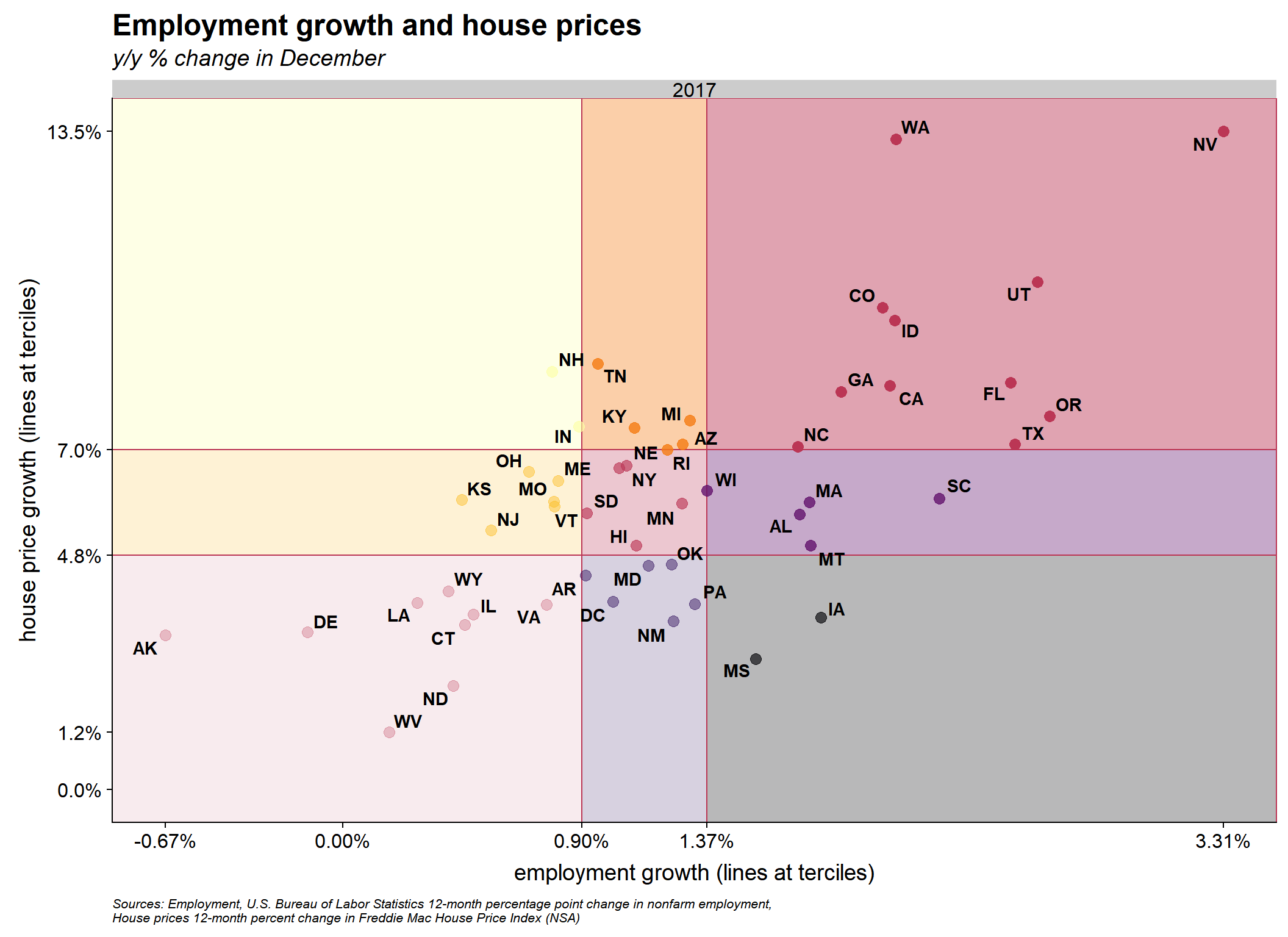
g.tile<-
  ggplot(data=dfb2,
         aes(x=EMPg,y=hpa,label=state,
             # see http://lenkiefer.com/2017/04/24/bivariate-map/
             # for explanation on the color/fill/alpha
             color=atan(y/x),
             fill=atan(y/x),
             alpha=x+y ))+
  geom_rect(aes(xmin=-Inf,xmax=Inf,ymin=-Inf,ymax=Inf,
                alpha=ifelse(state!="Legend",x+y,0)),color=NA)+
  # Draw gridlines to demarcate the terciles on the scatterplot
  geom_segment(aes(x=x0,xend=x3,y=hpa0,yend=hpa0),color="black")+
  geom_segment(aes(x=x0,xend=x3,y=hpa1,yend=hpa1),color="black")+
  geom_segment(aes(x=x0,xend=x3,y=hpa2,yend=hpa2),color="black")+
  geom_segment(aes(x=x0,xend=x3,y=hpa3,yend=hpa3),color="black")+
  geom_segment(aes(x=x0,xend=x0,y=hpa0,yend=hpa3),color="black")+
  geom_segment(aes(x=x1,xend=x1,y=hpa0,yend=hpa3),color="black")+
  geom_segment(aes(x=x2,xend=x2,y=hpa0,yend=hpa3),color="black")+
  geom_segment(aes(x=x3,xend=x3,y=hpa0,yend=hpa3),color="black")+

  # add a point to indicate where this state lies
  geom_point(alpha=1,color="black")+
  guides(fill=F,color=F,alpha=F)+
  scale_color_viridis(name="Color scale",option="B")+
  scale_fill_viridis(name="Color scale",option="B")+
  # Use geofacet::facet_geo to arrange the tiles
  facet_geo(~state, grid="us_state_grid1",label="code")  +
  theme(axis.text=element_blank(),
        plot.title=element_text(hjust=0,face="bold",size=18),
        plot.subtitle=element_text(hjust=0,face="italic",size=14),
        axis.ticks=element_blank(),
        axis.line=element_blank(),
        strip.background=element_blank(),
        panel.background=element_blank(),
        plot.background=element_rect(fill="white"),
        panel.grid.major = element_line(colour = NA),
        panel.grid.minor = element_line(colour = NA))+
  labs(x="",y="",title="Bivariate Tilegrid Map!",subtitle="@lenkiefer")

plot_grid(g.xy,g.tile,ncol=2)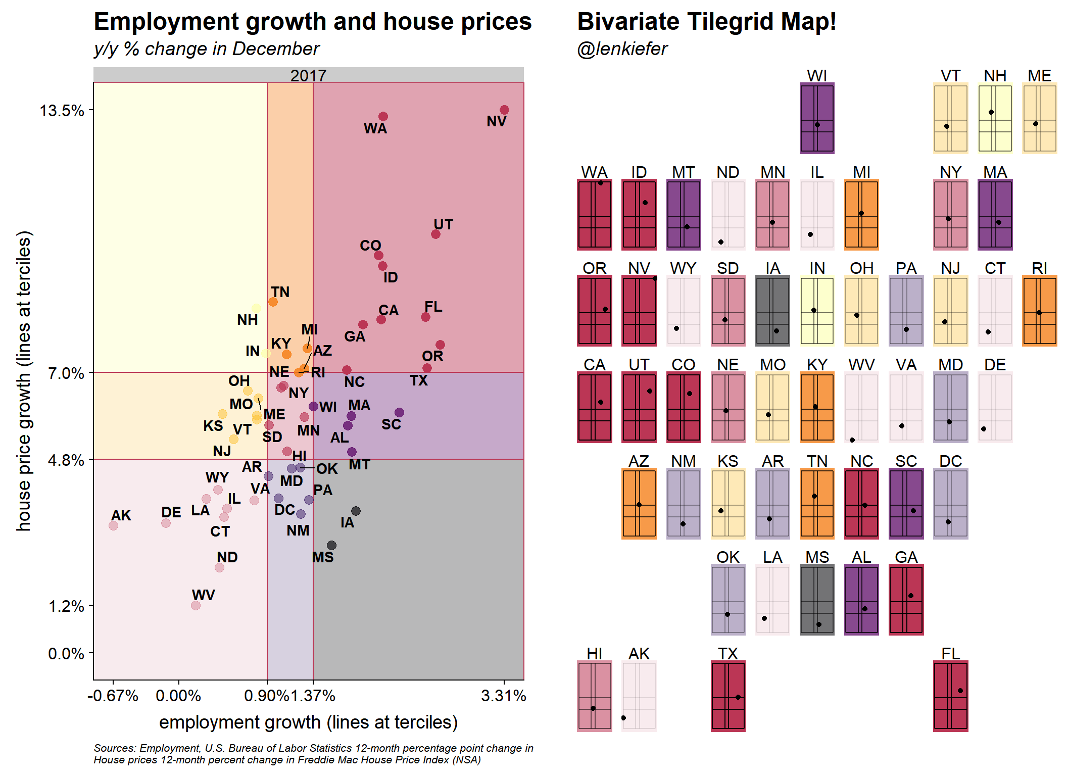
Discussion
I like this crazy plot. The scatterplot shows the relationship of house prices and employment, with those variables mapped to a bivariate color scale. The tilegrid map shows where the states are in the scatterplot with a stylized tile. Take Nevada (NV) for example. That state has the highest employment growth rate and the highest house price growth. In the tileplot, the dot for NV is in the top right corner. Alaska (AK) and West Virginia (WV) have the lowest employment and house price rates respectively and are thus on the left and bottom edges but not the corner.
Finally, let’s consider how the scatterplot has evolved over time:
ggplot(data=dfb,
       aes(x=EMPg,y=hpa,label=state,
           # see http://lenkiefer.com/2017/04/24/bivariate-map/
           # for explanation on the color/fill/alpha
           color=atan(y/x),
           fill=atan(y/x),
           alpha=x+y ))+

  # Shade areas based on the terciles
  geom_rect(data=dfq.all,aes(xmin=-Inf,xmax=x1,ymin=hpa1,ymax=hpa2,fill=atan(2/1),alpha=3/2))+
  geom_rect(data=dfq.all,aes(xmin=x1,xmax=x2,ymin=hpa1,ymax=hpa2,fill=atan(2/2),alpha=4/2))+
  geom_rect(data=dfq.all,aes(xmin=x2,xmax=Inf,ymin=hpa1,ymax=hpa2,fill=atan(2/3),alpha=5/2))+

  geom_rect(data=dfq.all,aes(xmin=-Inf,xmax=x1,ymin=-Inf,ymax=hpa1,fill=atan(1/1),alpha=2/2))+
  geom_rect(data=dfq.all,aes(xmin=x1,xmax=x2,ymin=-Inf,ymax=hpa1,fill=atan(1/2),alpha=3/2))+
  geom_rect(data=dfq.all,aes(xmin=x2,xmax=Inf,ymin=-Inf,ymax=hpa1,fill=atan(1/3),alpha=4/2))+

  geom_rect(data=dfq.all,aes(xmin=-Inf,xmax=x1,ymin=hpa2,ymax=Inf,fill=atan(3/1),alpha=4/2))+
  geom_rect(data=dfq.all,aes(xmin=x1,xmax=x2,ymin=hpa2,ymax=Inf, fill=atan(3/2),alpha=5/2))+
  geom_rect(data=dfq.all,aes(xmin=x2,xmax=Inf,ymin=hpa2,ymax=Inf, fill=atan(3/3),alpha=6/2))  +
  geom_point(size=3,shape=21)+
  scale_color_viridis(option="B")+
  scale_fill_viridis(option="B")+
  theme(legend.position="none",plot.title=element_text(hjust=0,face="bold",size=18),
        plot.subtitle=element_text(hjust=0,face="italic",size=14),
        plot.caption=element_text(hjust=0,size=8,face="italic"))+
  labs(x="employment growth",
       y="house price growth",
       title="Employment growth and house prices",
       subtitle="y/y % change in December",
       caption="Sources: Employment, U.S. Bureau of Labor Statistics 12-month percentage point change in nonfarm employment,\nHouse prices 12-month percent change in Freddie Mac House Price Index (NSA)")+
  scale_y_continuous(labels=percent)+
  scale_x_continuous(labels=percent)+
  facet_wrap(~year)
Here we see that while the relationship is generally positive, the slope tends to change. In the real world, there’s a lot more than employment growth going on in housing markets. However, in recent years employment growth serves as a reasonable proxy for demand growth. Thus we see a fairly strong and stable correlation between employment and house price trends over the past few years.
colors
I’m no expert on colors, but I’ve been playing around with different bivariate color schemes. Here are several I tried:
d<-expand.grid(x=1:100,y=1:100)

g.1<-
ggplot(d, aes(x,y,fill=atan(y/x),alpha=x+y))+
  geom_tile()+
  scale_fill_viridis()+
  theme(legend.position="none",
        panel.background=element_blank())+
  labs(title="Viridis",subtitle="A bivariate color scheme")

g.2<-
  ggplot(d, aes(x,y,fill=atan(y/x),alpha=x+y))+
  geom_tile()+
  scale_fill_distiller(palette = "RdYlGn",direction=1)  +
  theme(legend.position="none",
        panel.background=element_blank())+
  labs(title="Red Yellow Green: RdYlGn",subtitle="A bivariate color scheme")

g.3<-
  ggplot(d, aes(x,y,fill=atan(y/x),alpha=x+y))+
  geom_tile()+
  scale_fill_distiller(palette = "Spectral",direction=1)  +
  theme(legend.position="none",
        panel.background=element_blank())+
  labs(title="Spectral",subtitle="A bivariate color scheme")

g.4<-
  ggplot(d, aes(x,y,fill=atan(y/x),alpha=x+y))+
  geom_tile()+
  scale_fill_distiller(palette = "PuOr",direction=1)  +
  theme(legend.position="none",
        panel.background=element_blank())+
  labs(title="PuOr",subtitle="A bivariate color scheme")

g.5<-
  ggplot(d, aes(x,y,fill=atan(y/x),alpha=x+y))+
  geom_tile()+
  scale_fill_viridis(option="B")+
  theme(legend.position="none",
        panel.background=element_blank())+
  labs(title="viridis::Inferno",subtitle="A bivariate color scheme")

g.6<-
  ggplot(d, aes(x,y,fill=atan(y/x),alpha=x+y))+
  geom_tile()+
  scale_fill_viridis(option="B")+
  theme(legend.position="none",
        panel.background=element_blank())+
  labs(title="viridis::Magma",subtitle="A bivariate color scheme")

g.7<-
  ggplot(d, aes(x,y,fill=atan(y/x),alpha=x+y))+
  geom_tile()+
  scale_fill_viridis(option="C")+
  theme(legend.position="none",
        panel.background=element_blank())+
  labs(title="viridis::Plasma",subtitle="A bivariate color scheme")

g.8<-
  ggplot(d, aes(x,y,fill=atan(y/x),alpha=x+y))+
  geom_tile()+
  scale_fill_viridis(option="E")+
  theme(legend.position="none",
        panel.background=element_blank())+
  labs(title="viridis::Cividis",subtitle="A bivariate color scheme")

g.9<-
  ggplot(d, aes(x,y,fill=atan(y/x),alpha=x+y))+
  geom_tile()+
  scale_fill_distiller(palette = "RdGy")+
  theme(legend.position="none",
        panel.background=element_blank())+
  labs(title="RdGy",subtitle="A bivariate color scheme")

plot_grid(g.1,g.2,g.3,g.4,g.5,g.6,g.7,g.8,g.9+labs(caption="@lenkiefer"),align="hv")
Which do you like?