I’ve been thinking about how different macroeconomic shocks might affect the U.S. housing market. Given recent volatility it is hard to know how to size risks. But it could be a useful exercise to think through how certain typical shocks might impact the housing market.
Rather than take on a full structural approach, I just want to extend the reduced form VAR analysis we did in a post from last year.
In this example, I want to see how a shock to consumer sentiment, as measured by the University of Michigan’s Survey of Consumers might impact housing market activity.
Gather data, estimate VAR
Click for data wrangling code
library(tidyquant)
library(tidyverse)
library(vars)
library(patchwork)
tickers <- c("FEDFUNDS",
"GS10",
"MORTGAGE30US",
"UNRATE",
"PCEPILFE",
"HOUST",
"PCE",
"UMCSENT")
df <- tidyquant::tq_get(tickers,get="economic.data",from="1979-01-01") %>%
group_by(symbol,year=year(date),month=month(date)) %>%
summarize(price=last(price)) %>%
ungroup() %>%
mutate(date=as.Date(ISOdate(year,month,1)))
df2 <-
df %>%
pivot_wider(names_from=symbol,values_from=price) %>%
mutate(RPCE=PCE*first(PCEPILFE)/PCEPILFE,
PCE_INFLATION=PCEPILFE/lag(PCEPILFE)-1,
PCE_INFLATION12=PCEPILFE/lag(PCEPILFE,12)-1,
LOG_STARTS= log(HOUST),
FEDFUNDS=FEDFUNDS/100,
UNRATE=UNRATE/100,
GS10=GS10/100,
LOG_CONSUMER_SENTIMENT = log(UMCSENT )
) Click for estimation and plotting code
ts1 <- ts(df2[,c("LOG_STARTS","LOG_CONSUMER_SENTIMENT","UNRATE",
                 "PCE_INFLATION12","GS10","FEDFUNDS")],
          start=1979,frequency=12)

ts2 <- window(ts1,start=1980,end=2019+11/12)
var1 <- VAR(ts2, p=12,type="const")
irf1 <- irf(var1,n.ahead=60)
mycaption <- paste0("@lenkiefer Response estimated by VAR(12)",
"\nusing R package vars: https://CRAN.R-project.org/package=vars",
"\nResponse is based on six variable system with log Housing Starts, log Consumer sentiment Index,",
"\nUnemployment Rate, 12-month percent change in PCE core inflation, the 10-year U.S. Treasury Yield and the \nEffective Federal Funds Rate",
"\nMonthly data Jan 1980 to Dec 2019",
"\nSources: Census/HUD, BLS, BEA, University of Michigan, Federal Reserve",
"\nRetrieved from FRED, Federal Reserve Bank of St. Louis")
# code to make plots
myf <- function(i=1,j=2){
# hpa response of starts to consumer sentiment shock
irf_var1 <- data.frame(period=1:61,
low=irf1$Lower[[j]][,i],
up=irf1$Upper[[j]][,i],
m = irf1$irf[[j]][,i]
)
ggplot(data=irf_var1, aes(x=period,y=-m,ymin=-low,ymax=-up))+
geom_ribbon(fill="dodgerblue",alpha=0.5)+
geom_line(color="red")+
geom_hline(yintercept=0,linetype=2)+
theme(plot.caption=element_text(hjust=0))+
scale_y_continuous(labels=scales::percent)+
scale_x_continuous(breaks=seq(0,60,12))+
theme_minimal()+
theme(plot.caption=element_text(hjust=0))+
labs(x="months since shock",
y="Response",
title=paste0(colnames(ts2)[i]," response to ",colnames(ts2)[j], " shock"),
subtitle="Red line response, blue shaded area 95% sentiment interval")
}myf(1,2)+labs(caption=mycaption)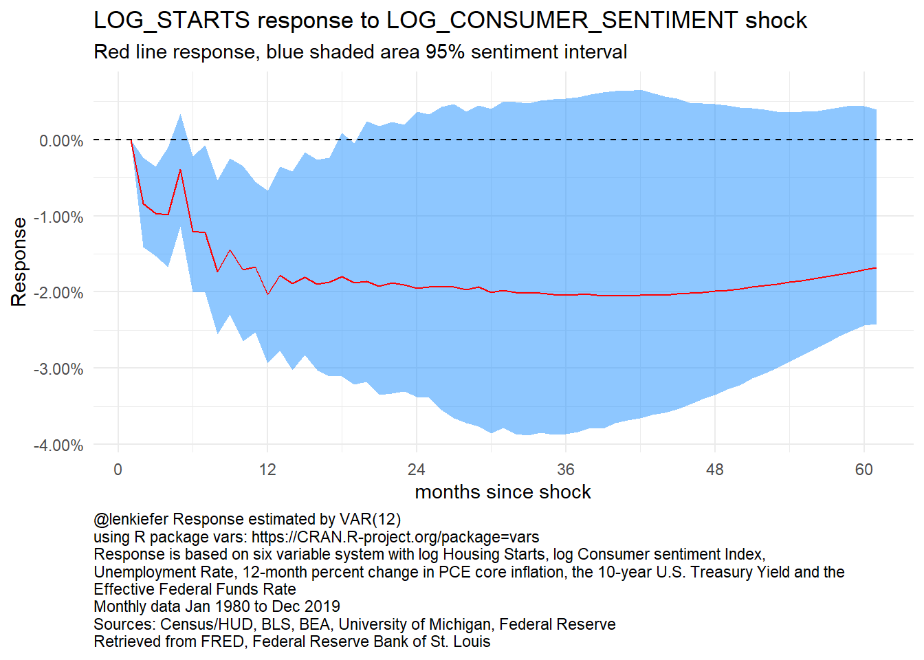
Figure 1: Impulse Response of Housing Starts to a Consumer Sentiment Shock
We can also use the R package patchwork to construct a composite plot:
myf(1,2)+labs(title="Housing Starts",subtitle="")+
myf(2,2)+labs(title="Consumer Sentiment",subtitle="") +
myf(3,2)+labs(title="Unemployment Rate",subtitle="") +
myf(4,2)+labs(title="Inflation",subtitle="") +
myf(5,2)+labs(title="10yr Treasury",subtitle="")+
myf(6,2)+labs(title="Fed Funds Rate",subtitle="") +
  plot_annotation(caption=mycaption,
                  title="Impulse Response to a Consumer Sentiment Shock",
                  theme = theme(plot.caption = element_text(hjust=0)))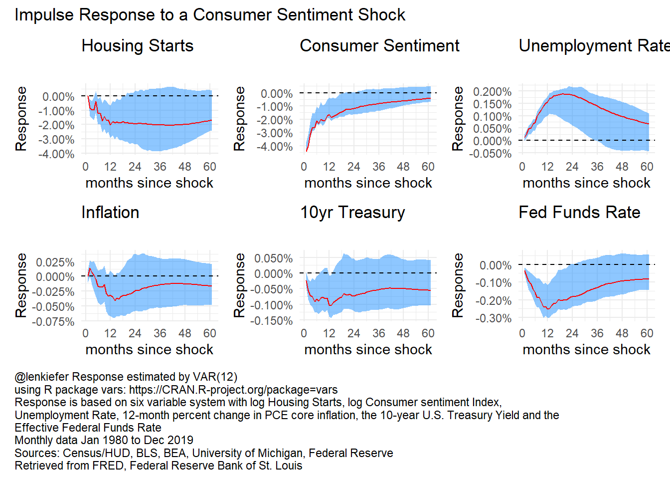
Figure 2: VAR IRF
These results look reasonable: a dip in consumer sentiment leads to a contraction in housing starts after about a year, unemployment rises a bit and fed accommodates with ~1 rate cut.
These results however assume a 4% decline in consumer sentiment (a typical/1 s.d. shock). As I tweeted out, during a recession the consumer sentiment index typically declines 20 to 30 percent:
consumer confidence index typically declines 20-30% (on y/y basis) during recession pic.twitter.com/1g5fK7Yv2W
— 📈 Len Kiefer 📊 (@lenkiefer) February 25, 2020
This type of reduced form analysis is far from complete. However, it does give us some sense of how changes in sentiment might impact the housing market. This could be a useful launching point for more careful analysis.