Mortgage interest rates have moved about a percentage point lower from where they were a year ago. The housing market seems to have responded favorably.
On my way into D.C. the other day to do some business, I joined a Twitter exchange originally between [at]Graykimbrough and Adam Ozimek, [at]ModeledBehavior about the effects of Federal Reserve interest policy on the housing market.
Seems unlikely housing market was slowed by trade war. That fed cuts have helped return it to growth suggest the hikes were to blame. Hard to call this the fed merely reacting to changing conditions. More like a mistake in hiking too fast too soon.
— Adam Ozimek (@ModeledBehavior) October 31, 2019
Adam has been of the view the Federal Reserve policy has been too tight, and one consequence of that was a slower housing market. Gray was a bit skeptical and brought up the (good) point that it was difficult to see through all the noise in various economic indicators. Was there really a positive response to recent Fed policy in the housing data?
For my part, I have been suggesting that lower mortgage rates, possibly due to Fed policy, but also possibly due to a bunch of other factors, has been benefiting the housing market recently. For example I have pointed out that the decline in mortgage rates has led a recovery in existing home sales.
lower mortgage rates have helped the U.S. housing market.
— 📈 Len Kiefer 📊 (@lenkiefer) October 28, 2019
After rates fell last fall, home sales stabilized. pic.twitter.com/DCBOfA0gsE
If we sharpen our pencils and do something a bit more formal than waving our hands really fast at a bunch of graphs, what do we get? Let’s explore.
Analytic game plan
In this post I’m going to do some formal analysis of the housing market and interest rates and see what we get. At a high level our approach will be:
- Get a bunch of macroeconomic data with as long of a time series as possible
- Estimate Vector AutoRegressions (VARs) to describe the dynamic correlations between variables
- Estimate the dynamic correlations using Linear Projections
- Consider an alternative identification strategy (sing restrictions) to the usual recursive identification scheme
The results won’t be conclusive, but they will provide some additional support for the claim that lower rates have benefited the housing market.
Per usual, I’ll share my R code to do the analysis, but this post will be more focused on the economics, so the R explanation will be in the comments or under a details tab.
Describing the Time Series
Let’s start with a brief explanation of our empirical approach. We’re going to use VARs or Local Projections to characterize the dynamics of a multivariate time series. Let \(Y_t\) denote a multivariate time series of \(m\) variables.
VAR Approach
We’ll describe the evolution of \(Y_t\) with the following equation:
\[ \begin{equation}\tag{1}A_0Y_t = \sum_{i=1}^k A_iY_{t-i} + \epsilon_t \end{equation}\]
We’d have trouble directly estimating the equation above, but we can much more easily estimate the following:
\[ \begin{equation}\tag{2}Y_t = \sum_{i=1}^k B_iY_{t-i} + u_t \end{equation}\]
Given estimates of \(B_i\) from equation (2) and some assumptions about \(u_t\) we might be able to recover the structural parameters \(A_0\),\(A_i\).
Lütkepohl, H. (2005) or Hamilton (1994) provide textbook treatments.
Local Projections Approach
Jorda (2005) suggests and alternative approach. Instead of estimating (2), we could instead estimate
\[ \begin{equation}\tag{3}Y_{t+s} = \sum_{i=1}^k C_iY_{t-i}+ \eta_t \end{equation}\]
Then under certain conditions we might be able to relate the coefficients \(C_i\) to the structural parameters \(A_0\),\(A_i\).
Data
We’re interested in relating interest rates (mortgage rates, Treasury yields and the federal funds rate), to housing market indicators. We’ll also need some control variables to account for the state of the economy. We’ll use a standard set of variables here. Specifically we’ll collect monthly data for the United State:
Macro Indicators
- Effective federal funds rate
- 10-year U.S. Treasury yield
- Unemployment rate
- Core PCE price index
- Personal consumption expenditures
Housing and Mortgage Market Variables
- Housing Starts (Total, SAAR 1000s)
- 30-year mortgage rate
- House price index (Freddie Mac U.S. house price index, seasonally adjusted)
- Mortgage debt outstanding (1-4 unit properties)
All of the economic variables are available from the St. Louis Federal Reserve Bank’s FRED.
We’ll also collect data on house prices (monthly) and mortgage rates (weekly) from Freddie Mac, and quarterly data on mortgage debt outstanding (MDO) from the Federal Reserve. All of these except for the house price index are also available from FRED.
The details tab provides information on how to gather these data. We’ll also perform a few data transformations.
Code to gather, wrangle data
# Load libraries
library(tidyverse)
library(forecast)
library(vars)
library(tsDyn)
library(lpirfs)
library(VARsignR)
library(lubridate)
library(tempdisagg)
library(cowplot)
library(data.table)
We are going to use several different R libraries to help us, including lpirfs, VARsignR, and tempdisagg.
# get house prices

dt <- data.table::fread('http://www.freddiemac.com/fmac-resources/research/docs/fmhpi_master_file.csv')

fmhpi <- dt[GEO_Type=="US",] %>% pull(Index_SA) %>% ts(start=1975,frequency=12) %>% log()

# get macro data
# FRED tickers

tickers <- c("FEDFUNDS",
             "GS10",
             "UNRATE",
             "PCEPILFE",
             "HOUST",
             "PCE")

# list of variable names
# SAAR is Seasonally Adjusted Annual Rate

vnames <-c("Effective Federal Funds Rate (%)",
           "10-year U.S. Treasury Yield (%, CMT)",
           "Unemployment Rate (%, SA)",
           "Core PCE Price Index (less food and energy, Index 2012=100, Seasonally Adjusted)",
           "Housing Starts (Total, SAAR 1000s)",
           "Personal Consumption Expenditure (Billions of Dollars, SAAR)")

df <- tidyquant::tq_get(tickers,get="economic.data",from="1959-01-01")
Now wrangle that data!
df2 <-
  df %>%
  pivot_wider(names_from=symbol,values_from=price)  %>%
  mutate(RPCE=PCE*first(PCEPILFE)/PCEPILFE,
         DRPCE = log(RPCE/lag(RPCE,1)),
         PCE_INFLATION=PCEPILFE/lag(PCEPILFE)-1,
         PCE_INFLATION12=PCEPILFE/lag(PCEPILFE,12)-1,
         LOG_STARTS= log(HOUST),
         FEDFUNDS=FEDFUNDS/100,
         UNRATE=UNRATE/100,
         GS10=GS10/100
         )

# house price growth (month/month)
hpa <-
  dt[GEO_Type=="US",] %>%
  pull(Index_SA) %>% ts(start=1975,frequency=12) %>%
  log() %>% diff() %>% window(start=1976)


# construct time series from monthly data, combine with house price data
ts1 <- ts(df2[,-1], start=1959,frequency=12)
ts2 <- ts.union(ts1,fmhpi, hpa)
colnames(ts2) <- c(colnames(ts1),"HPI","HPA")

# create real house price index
ts_temp <- ts.intersect(hpi=fmhpi,pce=log(ts2[,"PCEPILFE"]))
rhpi <- ts_temp[,"hpi"]-as.numeric(first(ts_temp[,"hpi"])) + as.numeric(first(ts_temp[,"pce"]))-ts_temp[,"pce"]

# mortgage rates, mortgage debt outstanding
df_mtgw <- tidyquant::tq_get("MORTGAGE30US",get="economic.data",from="1971-01-01")

# aggregate mortgage rate data to monthly
df_mtg <- df_mtgw %>% group_by(year=year(date),month=month(date)) %>%
  summarize(pmms30 = mean(price)) %>%ungroup()  %>% mutate(date=as.Date(ISOdate(year,month,1)))

pmms30 <- ts(df_mtg$pmms30, start=1971+3/12,frequency=12)

# quarterly MDO data
df_mdo <- tidyquant::tq_get("MDOTP1T4FR",get="economic.data",from="1950-01-01")
lmdo <- log(df_mdo$price) %>% ts(start=1950,frequency=4) %>% window(start=1960)
Converting quarterly to monthly data
Our default data frequency will be monthly data. Most of the data are already monthly. The mortgage rate data is weekly, but we can aggregate to monthly by taking the average of all weeks in the month as in the code above.
But the mortgage debt outstanding data comes to us quarterly via the Federal Reserve. We can use temporal disaggregation to interpolate the mortgage debt data using house prices. Details are below (click on the arrow in most browsers).
Interpolating quarterly data with tempdisagg
We could interpolate smoothly from quarterly to monthly assuming say a linear trend. But another approach would be to use indicator variables. We can relate the log level of MDO to the cumulative log sum of new home sales and the level of mortgage interest rates. The idea here is that cumulative total mortgage debt outstanding trends higher over time in proportion to the cumulative total of home sales.
ts4 <- ts.intersect(lmdo,aggregate(fmhpi,4,last))
cbind(mdo=ts4[,1]-as.numeric(first(ts4[,1]))+1, hpi=ts4[,2]-as.numeric(first(ts4[,2]))+1) %>%
  autoplot() + labs(x="date",y="index, 1975Q1= 1 ")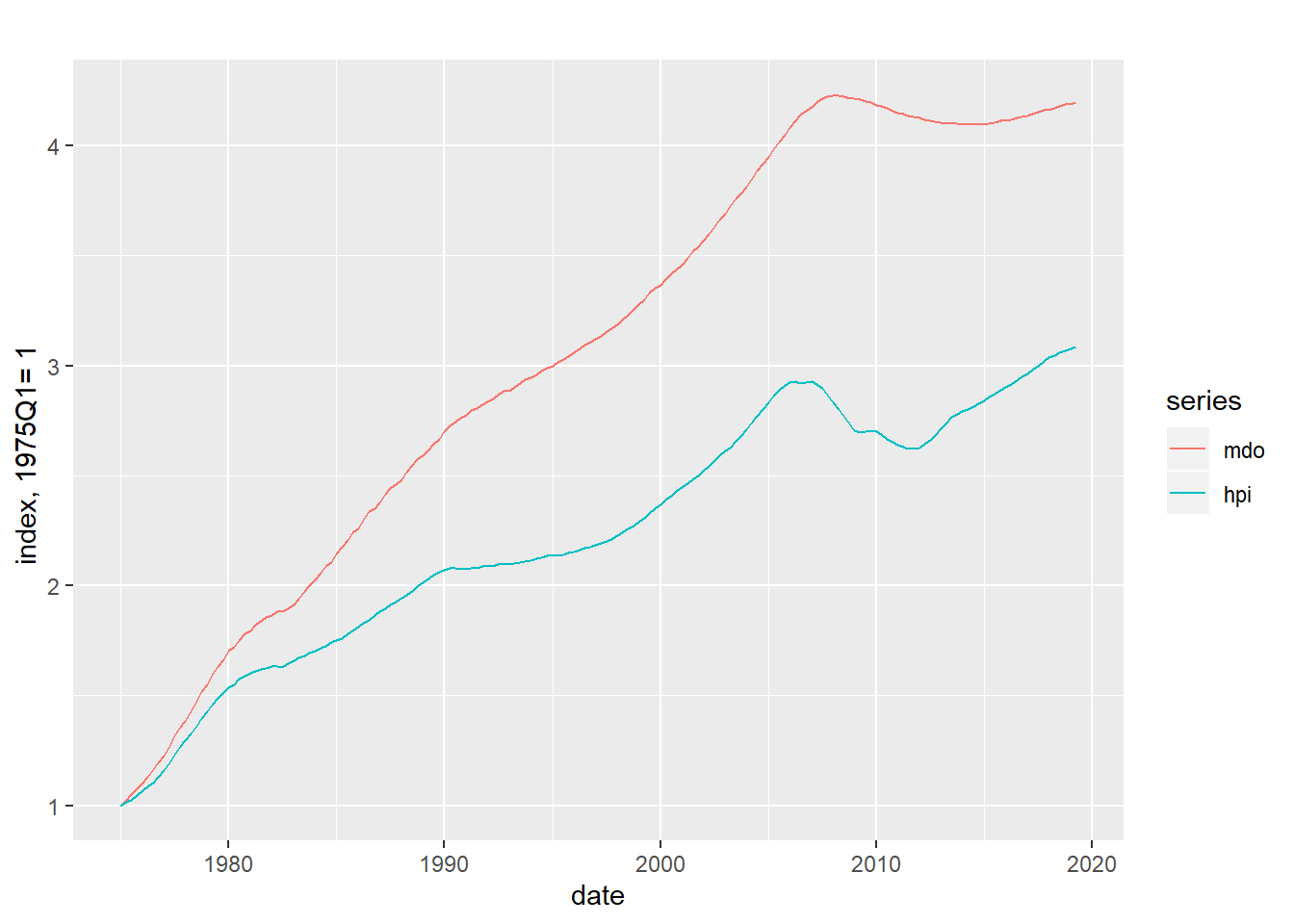
Figure 1: MDO and house pricess
# create monthly MDO series
td_fit <-  td(lmdo~fmhpi,conversion="last")
## Warning in td(lmdo ~ fmhpi, conversion = "last"): High frequency series
## shorter than low frequency. Low frequency values from 1975 are used.summary(td_fit)##
## Call:
## td(formula = lmdo ~ fmhpi, conversion = "last")
##
## Residuals:
## Min 1Q Median 3Q Max
## -0.5499 -0.1443 0.3181 0.4938 0.8684
##
## Coefficients:
## Estimate Std. Error t value Pr(>|t|)
## (Intercept) 10.19526 0.29796 34.22 <2e-16 ***
## fmhpi 1.05986 0.05776 18.35 <2e-16 ***
## ---
## Signif. codes: 0 '***' 0.001 '**' 0.01 '*' 0.05 '.' 0.1 ' ' 1
##
## 'chow-lin-maxlog' disaggregation with 'last' conversion
## 178 low-freq. obs. converted to 537 high-freq. obs.
## Adjusted R-squared: 0.6548 AR1-Parameter: 0.999The results aboves suggest that for every 1 percent increase in house prices mortgage debt outstanding increases by a little over 1 percent. For this interpolation we require that log house prices are cointegrated with log mortgage debt outstanding.
Even if that’s not true (the AR parameter of 0.999 might be an issue) the interpolation is pretty smooth so this does relatively little violence to the data as we see in the plot below.
log_mdo <- td_fit %>% predict()
autoplot(log_mdo) + autolayer(lmdo,color="red")+
  labs(title="Log MDO and monthly interpolation",
       caption="Interpolation based on temporal disaggration of Log MDO ~ Log House Prices")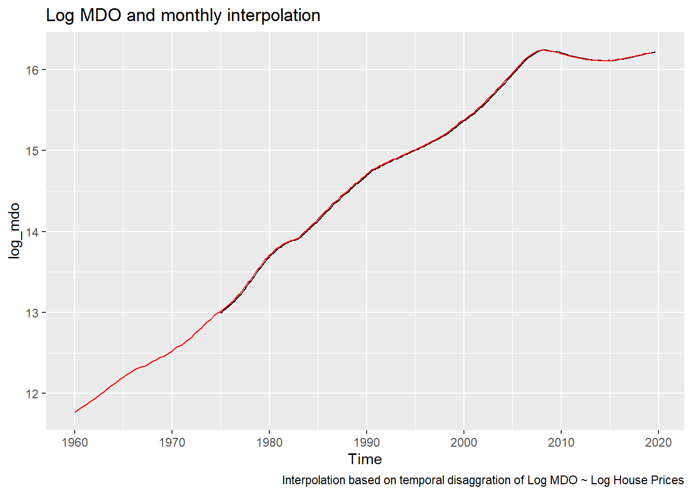
Figure 2: Interpolating Monthly MDO
ts3 <- ts.union(ts2,pmms30/100,log_mdo)
colnames(ts3) <- c(colnames(ts2),"MORTGAGE_RATE","LOG_MDO")
We could refine this more later, but since MDO is only of tertiary concern here we’ll move on for now.
Summarize that data
Before we get into the regressions and stuff, let’s look at our data. Specifically, let’s plot the paths for the effective federal funds rate, the 30-year mortgage rate and housing starts.
g1 <- autoplot(ts3[,"FEDFUNDS"]*100)+labs(x="",y="",title="Effective Federal Funds Rate (%)")
g2 <- autoplot(ts3[,"MORTGAGE_RATE"]*100)+labs(x="",y="",title="30-year Fixed Mortgage Rate (%)")
g3 <- autoplot(ts3[,"HOUST"])+labs(x="",y="",title="Housing Starts (1000s, SAAR)")
plot_grid(g1,g2,g3,ncol=1)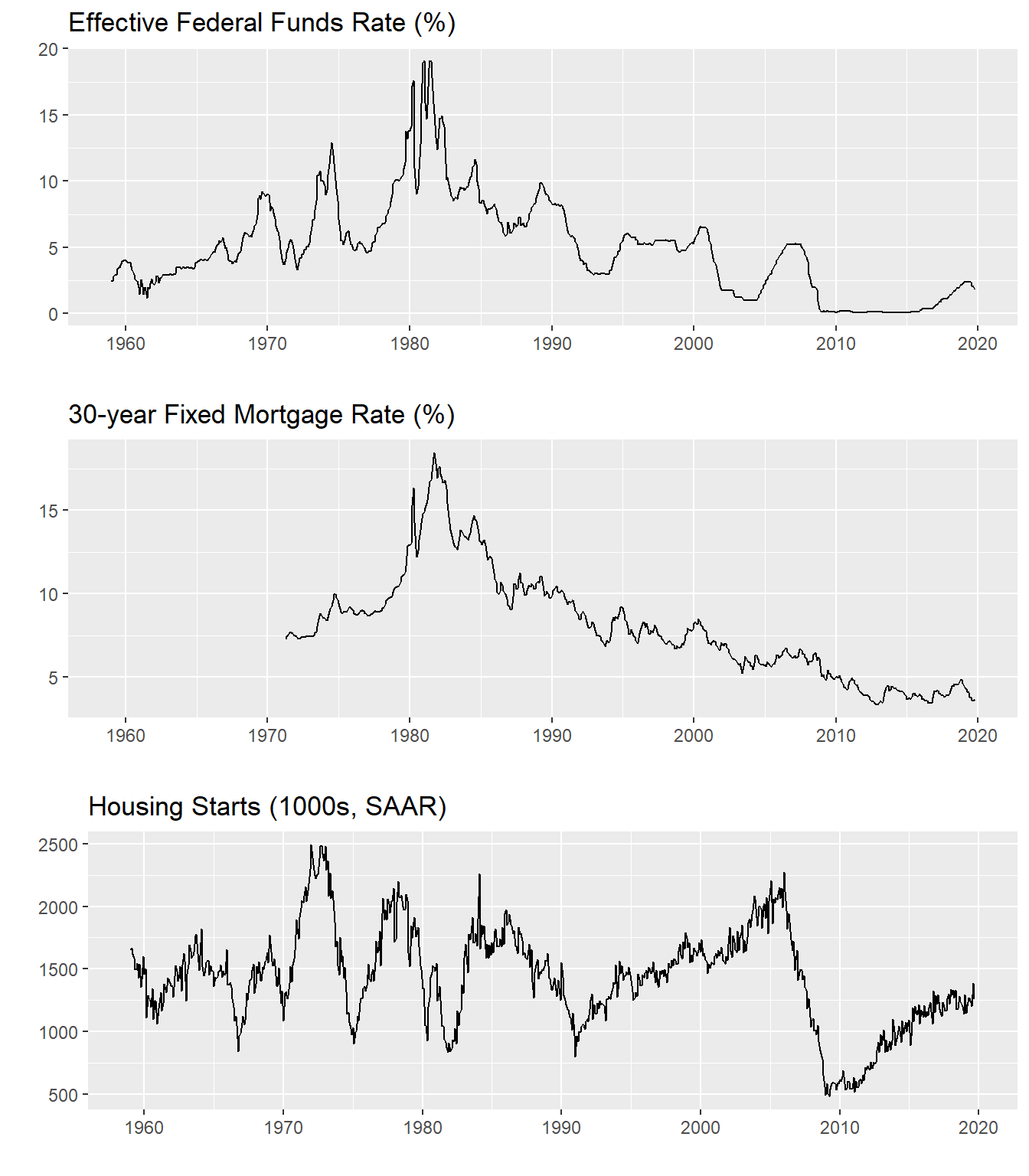
Figure 3: Trends in fed funds rate, mortgage rate, housing starts
Is there a relationship between interest rates and housing starts? Perhaps, let’s construct a scatterplot with 1-month changes in mortgage interest rates on the x axis and 1-month changes in log starts on the y axis (approximately equal to percent changes in starts).
ggplot(data=NULL,
       aes(x=diff(ts3[,"MORTGAGE_RATE"]),
           y=diff(log(ts3[,"HOUST"])))) +
  geom_point()+stat_smooth(method="lm",fill=NA)+
  labs(x="change in mortgage rate",y="change in Log(Housing Starts)",
       title="Changes in mortgage rates and log(housing starts)")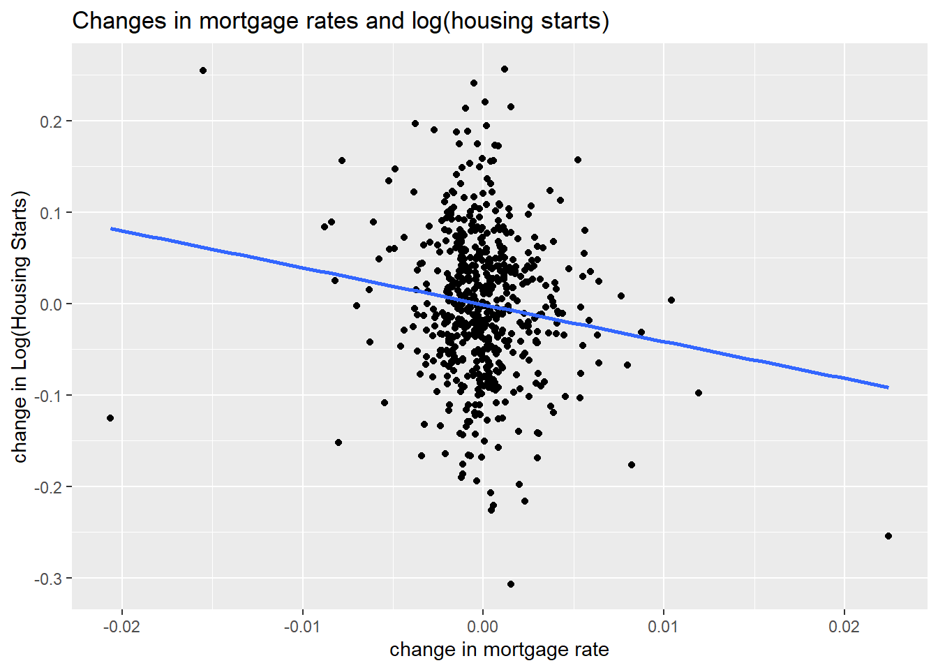
Figure 4: When interest rates increase, housing starts fall
out<- lm(diff(log(ts3[,"HOUST"]))~diff(ts3[,"MORTGAGE_RATE"]))
stargazer::stargazer(out, type="html",
                     title="Linear Regression: Change in Log_Starts ~ Change in Mortgage Rate",
                     dep.var.labels=c("Change in Log Housing Starts"),
covariate.labels=c("Change in Mortgage Rate"))| Dependent variable: | |
| Change in Log Housing Starts | |
| Change in Mortgage Rate | -4.042*** |
| (1.195) | |
| Constant | -0.001 |
| (0.003) | |
| Observations | 581 |
| R2 | 0.019 |
| Adjusted R2 | 0.018 |
| Residual Std. Error | 0.079 (df = 579) |
| F Statistic | 11.442*** (df = 1; 579) |
| Note: | p<0.1; p<0.05; p<0.01 |
According to the linear regression every 1 percentage point increase in mortgage rates is associated with a 4 percent decrease in housing starts.
This is some evidence for contemporaneous correlation, but far from causal. It could be that lower housing starts are causing higher mortgage rates (weird, but we can’t rule it out a priori) or perhaps a third variable is causing both.
To get closer to causality—to show that higher rates slow housing market activity—we need to establish two things. First, that changes in mortgage rates lead declines in housing market activity. Second, and quite a bit harder, rule out other factors that might be driving both variables.
It seems quite intuitive that changes in the mortgage rate should lead lower housing starts. But if you want to see some evidence, see below the fold here.
Showing mortgage rate changes lead housing starts
We can demonstrate that changes in the mortgage rate lead changes in log starts and not vice versa via the cross correlation function (CCF) and Granger Causality tests. First, let’s plot the CCF.
drate=diff(ts3[,"MORTGAGE_RATE"])
dlog_starts=diff(log(ts3[,"HOUST"]))
ccf(drate,dlog_starts,na.action=na.exclude, main="Cross Correlation Function: Change Mortgage Rate & Change Log Starts")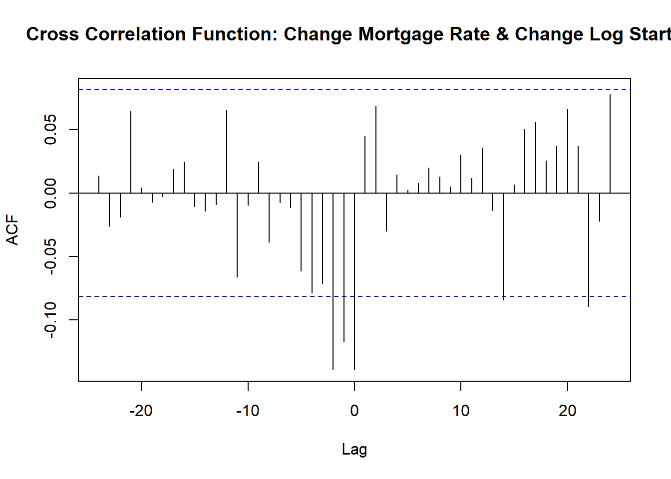
Figure 5: Cross correlation function of changes in mortgage rates and changes in log starts
The CCF shows that changes in the mortgage rate are lead changes in log starts by two to three months.
We can also conduct a bivariate Granger Causality test:
grangertest(drate, dlog_starts, order = 12, na.action = na.omit)## Granger causality test
##
## Model 1: dlog_starts ~ Lags(dlog_starts, 1:12) + Lags(drate, 1:12)
## Model 2: dlog_starts ~ Lags(dlog_starts, 1:12)
## Res.Df Df F Pr(>F)
## 1 544
## 2 556 -12 5.2051 2.597e-08 ***
## ---
## Signif. codes: 0 '***' 0.001 '**' 0.01 '*' 0.05 '.' 0.1 ' ' 1grangertest( dlog_starts,drate, order = 12, na.action = na.omit)## Granger causality test
##
## Model 1: drate ~ Lags(drate, 1:12) + Lags(dlog_starts, 1:12)
## Model 2: drate ~ Lags(drate, 1:12)
## Res.Df Df F Pr(>F)
## 1 544
## 2 556 -12 1.0531 0.3983The Granger Causality tests show that changes in the mortgage rate provide useful information about future changes in log housing starts even after controlling for the recent history of housing starts. The second set shows that log housing starts does not Granger cause changes in mortgage rates.
Controlling for other factors
We’ve shown that change in mortgage rates lead changes in housing starts and not vice versa, but what about other confounding factors? Here is where the VAR might help. By including other variables that control for economic conditions we can try to isolate the impact of rates on housing activity.
Standard VAR with recursive identification
Let’s estimate a VAR with the following 5 variables (in this order)
- Log housing starts
- Unemployment rate
- 12-month percent change in Core PCE inflation
- 10-year U.S. Treasury yield
- Effective federal funds rate
R code to estimate VAR,make plots
ts5 <- ts2[,c("LOG_STARTS","UNRATE","PCE_INFLATION12","GS10","FEDFUNDS")]
var1 <- VAR(ts5 %>% window(start=1960,end=2019+8/12), p=12,type="const")
irf1 <- irf(var1,n.ahead=60)
# collect responses as data frame (for plotting)

# response of starts to fed funds
irf_var1 <- data.frame(period=1:61,
                       low=irf1$Lower[[5]][,1],
                       up=irf1$Upper[[5]][,1],
                       m = irf1$irf[[5]][,1]
                       )
# response of starts to 10-year Treasury
irf_var2 <- data.frame(period=1:61,
                       low=irf1$Lower[[4]][,1],
                       up=irf1$Upper[[4]][,1],
                       m = irf1$irf[[4]][,1]
)

# plot response of starts to Fed Funds

irf_plot1 <-
ggplot(data=irf_var1, aes(x=period,y=m,ymin=low,ymax=up))+
  geom_ribbon(fill="dodgerblue",alpha=0.5)+
  geom_line(color="red")+
  geom_hline(yintercept=0,linetype=2)+
  theme(plot.caption=element_text(hjust=0))+
  scale_y_continuous(labels=scales::percent)+
  scale_x_continuous(breaks=seq(0,60,12))+
  labs(x="months since shock",
       y="Response of log starts (% change in starts)",
       title="Housing Starts Response to FEDFUNDS Shock",
       subtitle="Red line response, blue shaded area 95% confidence interval",
       caption=paste0("@lenkiefer Response estimated by VAR. Response of LOG_STARTS to 1 s.d. FEDFUNDS shock",
                      "\nusing R pacake vars: https://CRAN.R-project.org/package=vars",
                      "\nResponse is based on five variable system with Log Housing Starts, Unemployment Rate,",
                      #"Monthly Change in INdustrial Production",
                      "\n12-month percent change in PCE core inflation, the 10-year U.S. Treasury Yield and the Effective Federal Funds Rate",
                      "\nMonthly data Jan 1960 to Sep 2019",
                      "\nSources: Census/HUD, BLS, BEA, Federal Reserve",
                      "\nRetrieved from FRED, Federal Reserve Bank of St. Louis"))

# plot response of starts to 10-year Treasury

irf_plot2<-
  ggplot(data=irf_var2, aes(x=period,y=m,ymin=low,ymax=up))+
  geom_ribbon(fill="dodgerblue",alpha=0.5)+
  geom_line(color="red")+
  geom_hline(yintercept=0,linetype=2)+
  theme(plot.caption=element_text(hjust=0))+
  scale_y_continuous(labels=scales::percent)+
  scale_x_continuous(breaks=seq(0,60,12))+
  labs(x="months since shock",
       y="Response of log starts (% change in starts)",
       title="Housing Starts Response to 10-year Treasury Shock",
       subtitle="Red line response, blue shaded area 95% confidence interval",
       caption=paste0("@lenkiefer Response estimated by VAR. Response of LOG_STARTS to 1 s.d. 10-year Treasury shock",
                      "\nusing R pacake vars: https://CRAN.R-project.org/package=vars",
                      "\nResponse is based on five variable system with Log Housing Starts, Unemployment Rate,",
                      #"Monthly Change in INdustrial Production",
                      "\n12-month percent change in PCE core inflation, the 10-year U.S. Treasury Yield and the Effective Federal Funds Rate",
                      "\nMonthly data Jan 1960 to Sep 2019",
                      "\nSources: Census/HUD, BLS, BEA, Federal Reserve",
                      "\nRetrieved from FRED, Federal Reserve Bank of St. Louis"))
VAR results are hard to consume. With 12 lags, 5 variables and 5 intercepts we have 65 parameters summarizing the dynamics of these variables. A standard practice is to compute an impulse response function.
Let’s examine the impulse response based on this VAR. We’ll first look a the response of log housing starts to a 1 standard deviation shock to the effective federal funds rate.
irf_plot1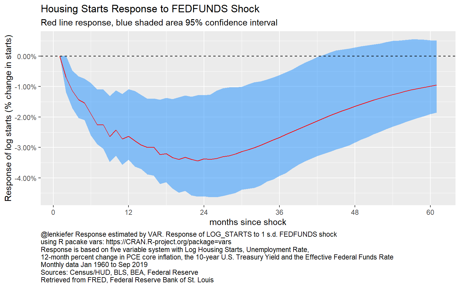
Figure 6: Impulse Response of Log Starts to a Federal Funds Rate Shock: VAR
This chart shows the response of log housing starts to a 1 standard deviation (about 25 basis points) shock to the federal funds rate over 60 months. The bands are quite wide, representing the uncertainty in the estimates. But even given the uncertainty, it’s clear that higher federal funds rate lead to lower housing starts. A year following a one standard deviation shock to the federal funds rate, housing starts have declined about 3 percent. Gradually, over time housing starts recover, but even after 5 years the point estimates has a 1 percent decline ins tarts.
Now let’s examine the response to a 1 standard deviation shock to the 10-year Treasury rate.
# plot VAR response
irf_plot2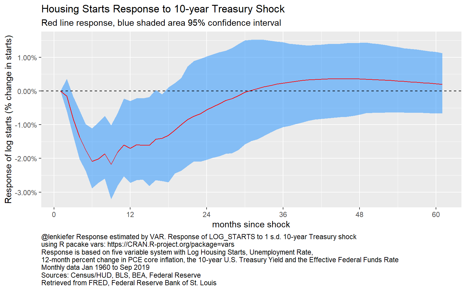
Figure 7: Impulse Response of Log Starts to a 10-year Treasury shock
Here we see a more immediate but shallower response. Following a shock to the 10-year Treasury rate housing starts decline by about 2 percent. The effects fade faster, returning to 0 after two and a half years.
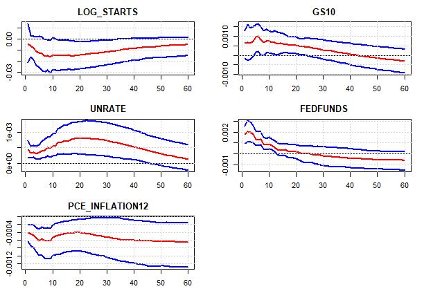
We don’t plot all the rest of the VAR responses out here, but you can see them in the details below.
All VAR responses
plot(irf1 )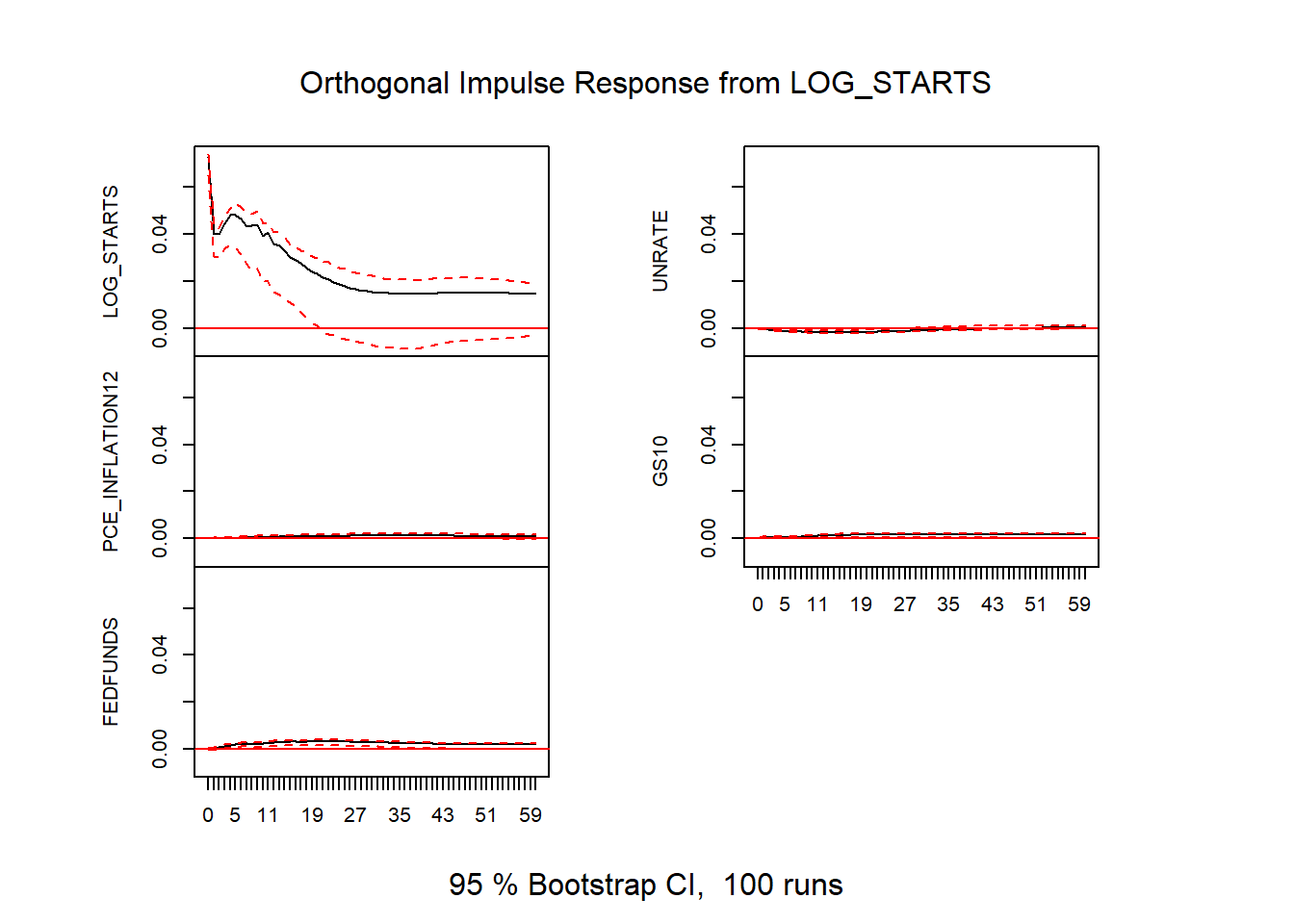
Figure 8: VAR impulse responses
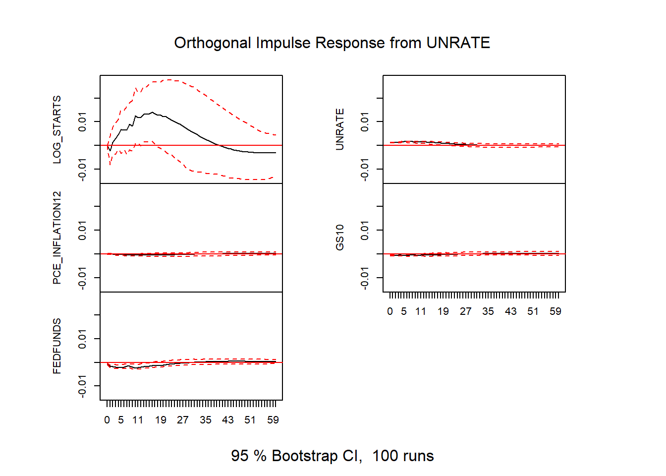
Figure 9: VAR impulse responses
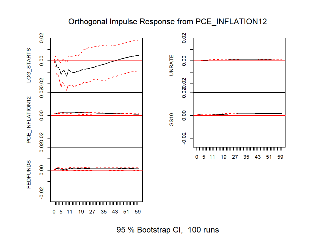
Figure 10: VAR impulse responses
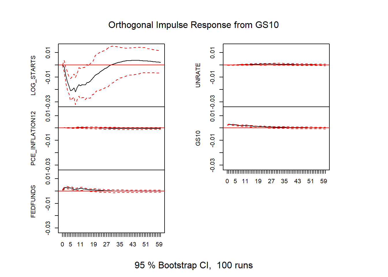
Figure 11: VAR impulse responses
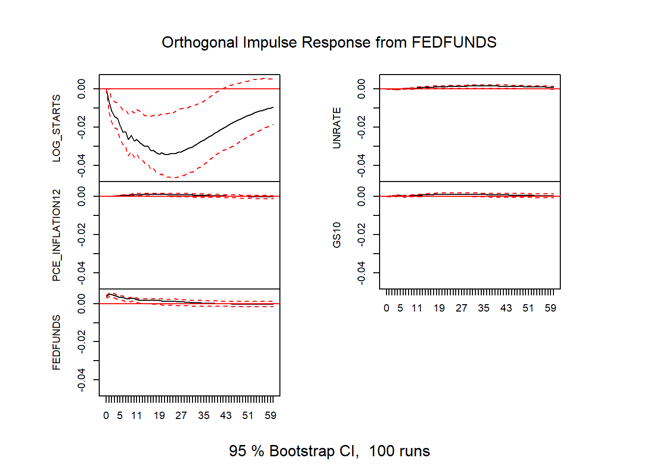
Figure 12: VAR impulse responses
Issues with standard VAR Impulse Response Functions
These standard VAR impulse responses only identify a meaningful shock insofar as the recursive ordering holds. In this case, we require that housing starts, ordered last, only responds to economic conditions and interest rates with a lag. Given that it takes about a month from permit to start this restriction doesn’t seem too unrealistic. But we’ll consider an alternative identification below.
There’s another issue, the VAR may be misspecfiied. If the VAR is misspecified then the impulse responses aren’t very useful. For example, we might have estimated a VAR with the wrong number of lags. We used 12 lags here, but perhaps we should have used 6 lags.
One way around possible misspecification is to use local projections.
Local Projections Estimates
We can estimate local projections using the R package lpirfs. R code to estimate Local Projections,make plots
results_lin <- lp_lin(data.frame(ts5),
                      lags_endog_lin=12,
                      trend=0,
                      shock_type=0,
                      confint=1.96,
                      hor=60)

outp <- plot_lin(results_lin)[[5]]

dfp <-
  data.frame(period=1:61,
           m = results_lin$irf_lin_mean[1, , 5],
           low = results_lin$irf_lin_low[1, , 5],
           up = results_lin$irf_lin_up[1, , 5]
           )
# LPIRF Starts to FED Funds
g_lpirf <-
  ggplot(data=dfp, aes(x=period,y=m,ymin=low,ymax=up))+
  geom_ribbon(fill="dodgerblue",alpha=0.5)+
  geom_line(color="red")+
  geom_hline(yintercept=0,linetype=2)+
  theme(plot.caption=element_text(hjust=0))+
  scale_y_continuous(labels=scales::percent)+
  scale_x_continuous(breaks=seq(0,60,12))+
  labs(x="months since shock",
       y="Response of log starts (% change in starts)",
       title="Housing Starts Response to FEDFUNDS Shock",
       subtitle="Red line response, blue shaded area 95% confidence interval",
       caption=paste0("@lenkiefer Response estimated by Local Projections. Response of LOG_STARTS to 1 s.d. FEDFUNDS shock",
                      "\nusing R pacake lpirfs: https://CRAN.R-project.org/package=lpirfs",
                      "\nResponse is based on five variable system with Log Housing Starts, Unemployment Rate,",
                      #"Monthly Change in INdustrial Production",
                      "\n12-month percent change in PCE core inflation, the 10-year U.S. Treasury Yield and the Effective Federal Funds Rate",
                      "\nSources: Census/HUD, BLS, BEA, Federal Reserve",
                      "\nRetrieved from FRED, Federal Reserve Bank of St. Louis"))


dfp2 <-
  data.frame(period=1:61,
           m = results_lin$irf_lin_mean[1, , 4],
           low = results_lin$irf_lin_low[1, , 4],
           up = results_lin$irf_lin_up[1, , 4]
           )
# LPIRF Starts to 10-year Treasury rate
g_lpirf2 <-
  ggplot(data=dfp2, aes(x=period,y=m,ymin=low,ymax=up))+
  geom_ribbon(fill="dodgerblue",alpha=0.5)+
  geom_line(color="red")+
  geom_hline(yintercept=0,linetype=2)+
  theme(plot.caption=element_text(hjust=0))+
  scale_y_continuous(labels=scales::percent)+
  scale_x_continuous(breaks=seq(0,60,12))+
  labs(x="months since shock",
       y="Response of log starts (% change in starts)",
       title="Housing Starts Response to 10-year Treasury Shock",
       subtitle="Red line response, blue shaded area 95% confidence interval",
       caption=paste0("@lenkiefer Response estimated by Local Projections. Response of LOG_STARTS to 1 s.d. 10-year Treasury shock",
                      "\nusing R pacake lpirfs: https://CRAN.R-project.org/package=lpirfs",
                      "\nResponse is based on five variable system with Log Housing Starts, Unemployment Rate,",
                      #"Monthly Change in INdustrial Production",
                      "\n12-month percent change in PCE core inflation, the 10-year U.S. Treasury Yield and the Effective Federal Funds Rate",
                      "\nSources: Census/HUD, BLS, BEA, Federal Reserve",
                      "\nRetrieved from FRED, Federal Reserve Bank of St. Louis"))
g_lpirf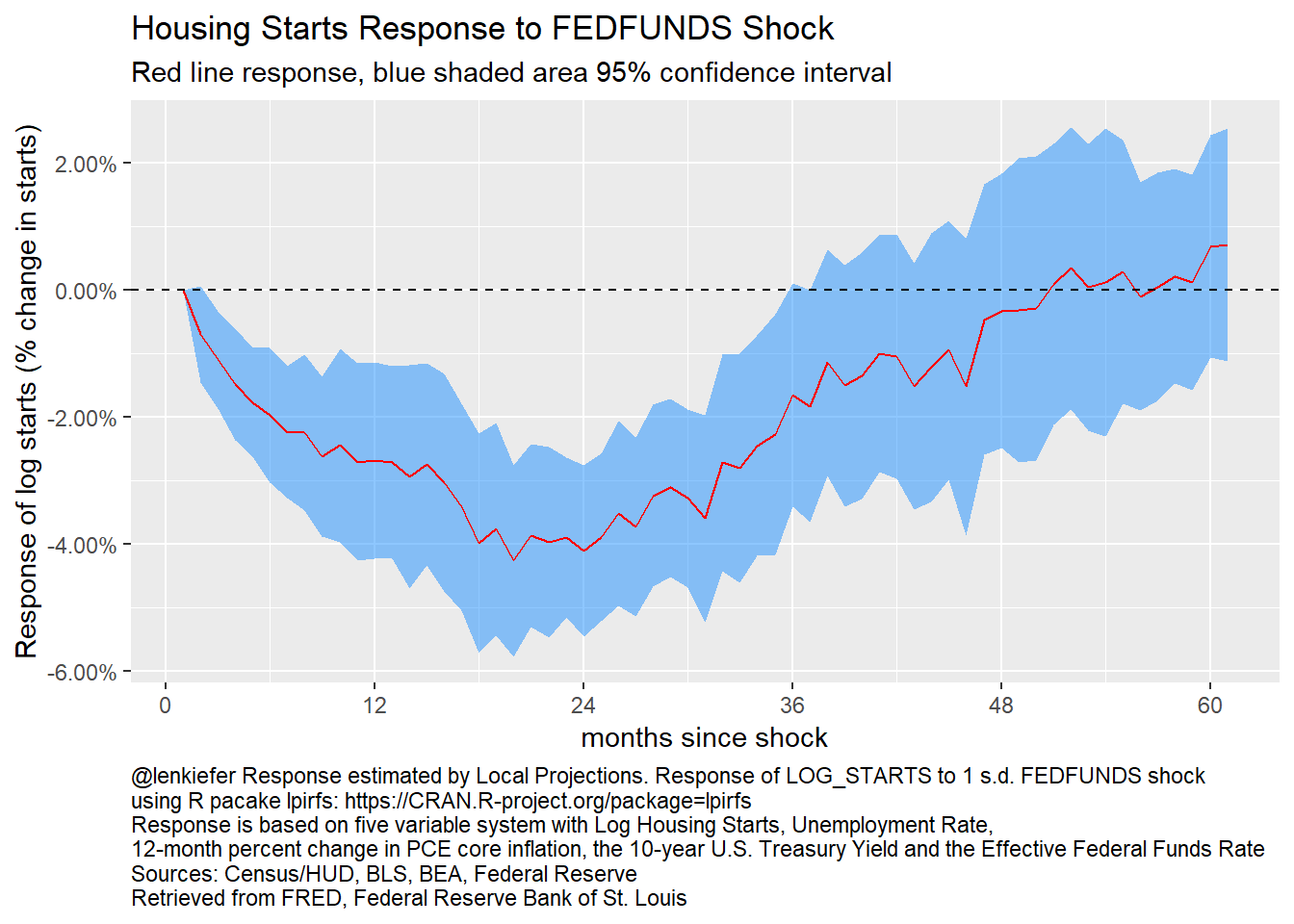
Figure 13: Local Projections: Response of log starts to fed funds shock
The local projections impulse response function for housing starts to a fed funds shock looks similar to the one we estimated with the VAR. In this case housing starts decline about 4 percent after a year and a half. Ater 4 years the response returns to zero.
g_lpirf2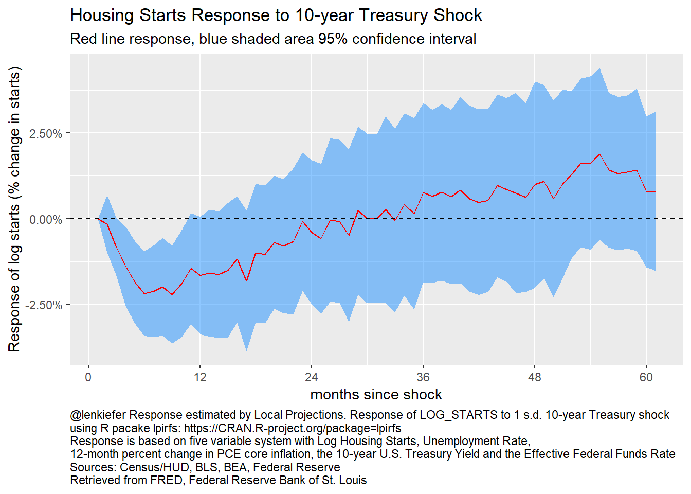
Figure 14: Local Projections: Response of log starts to 10-year Treasury shock
As with the response to the federal funds rate shock, the local projection impulse response of housing starts to a 10-year Treasury shock looks similar to the VAR reponse function.
Sign Restrictions
An alternative to the reursive restrictions is the use of sign restrictions. See for example Fry and Pagan (2011) for useful discussion. We can estimate impulse responses using sign restrictions with the VARsignR package.
We can bring some a priori restrictions to the possible impulse responses to uncover something closer to the true impulse response.
Here we will assume that a federal funds rate shock:
- Increase the fed funds rate for 12 months
- Decreases core inflation for 12 months
- Increase the unemployment rate for 12 months
We can look for impulse response functions that satisfy these responses and plot them. The code in the details tabe below does that for us.
R code for VAR with sign restrictions
# sign restrictions on VAR responses
constr <- c(+5,-3,+2)
model1 <- uhlig.reject(Y=ts5 %>% window(start=1960,end=2019+8/12),
                       nlags=12, draws=200, subdraws=200, nkeep=1000,
                       KMIN=1,
                       KMAX=12,  #restrictions hold for 12 months
                       constrained=constr, constant=TRUE, steps=60)
irfs1 <- model1$IRFS
vl <-colnames(ts5)

# call this to save plot (without comments)

irfplot(irfdraws=irfs1, type="median",
        labels=vl,
        save=TRUE,
        bands=c(0.16, 0.84),
       grid=TRUE, bw=FALSE)
Here’s the resulting figure:
In this figure we plot the response in red along with 68 percent bands. The area between the blue lines represent the range of impulse responses given our estimated VAR that are consistent with our sign restrictions. In this case we see the line for housing starts goes negative to about 2 percent after a year, very similar to the basline estimates for the VAR with recursive identification and the local proejections impulse responses.
Unlike with the two prior approaches, the sign restriciton (as implemented in R) can only identify the response to a single shock. While the bands are different the general shape of the response of impulse response functions are similar across all methods. Following a shock to the fed funds rate, housing starts decline.
How do other housing variables respond to higher interest rates?
What about other housing variables?
We could also try to include additional controls. We can extend the VAR as in Musso, Neri, Stracca (2011). Using monthly data we now estimate a seven variable system
- Core PCE price index (log level)
- Real consumption (log level)
- Log housing starts
- Real house Price index (Freddie Mac US Index deflated by Core PCE price index)
- Federal funds rate
- 30-year fixed mortgage rate
- Log mortgage debt outstanding
The details tab below has the R code to estimate the 7 variable VAR along with the impulse responses for all variables in the system (49 plots). Below we will draw bigger plots for a couple impulse responses and discuss.
R code for and many plots for VAR
# same as in https://www.econstor.eu/bitstream/10419/153595/1/ecbwp1161.pdf
ts6 <- ts.intersect(pce_core_index=log(ts2[,"PCEPILFE"]),
                    real_consumption=log(ts2[,"RPCE"]),
                    log_starts=ts2[,"LOG_STARTS"],
                    real_house_price=rhpi,
                    fedfunds=ts5[,"FEDFUNDS"],
                    mtg_rate=pmms30/100,
                    log_mdo)

var6 <- VAR(ts6, p=12,type="const")
irf6 <- irf(var6,n.ahead=60)
plot(irf6)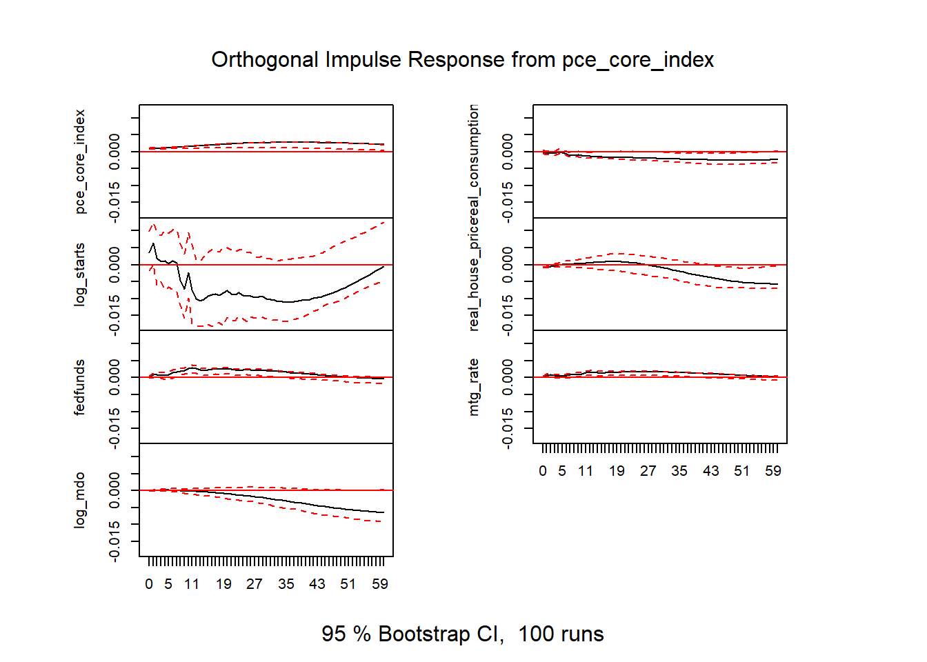
Figure 15: VAR results v2
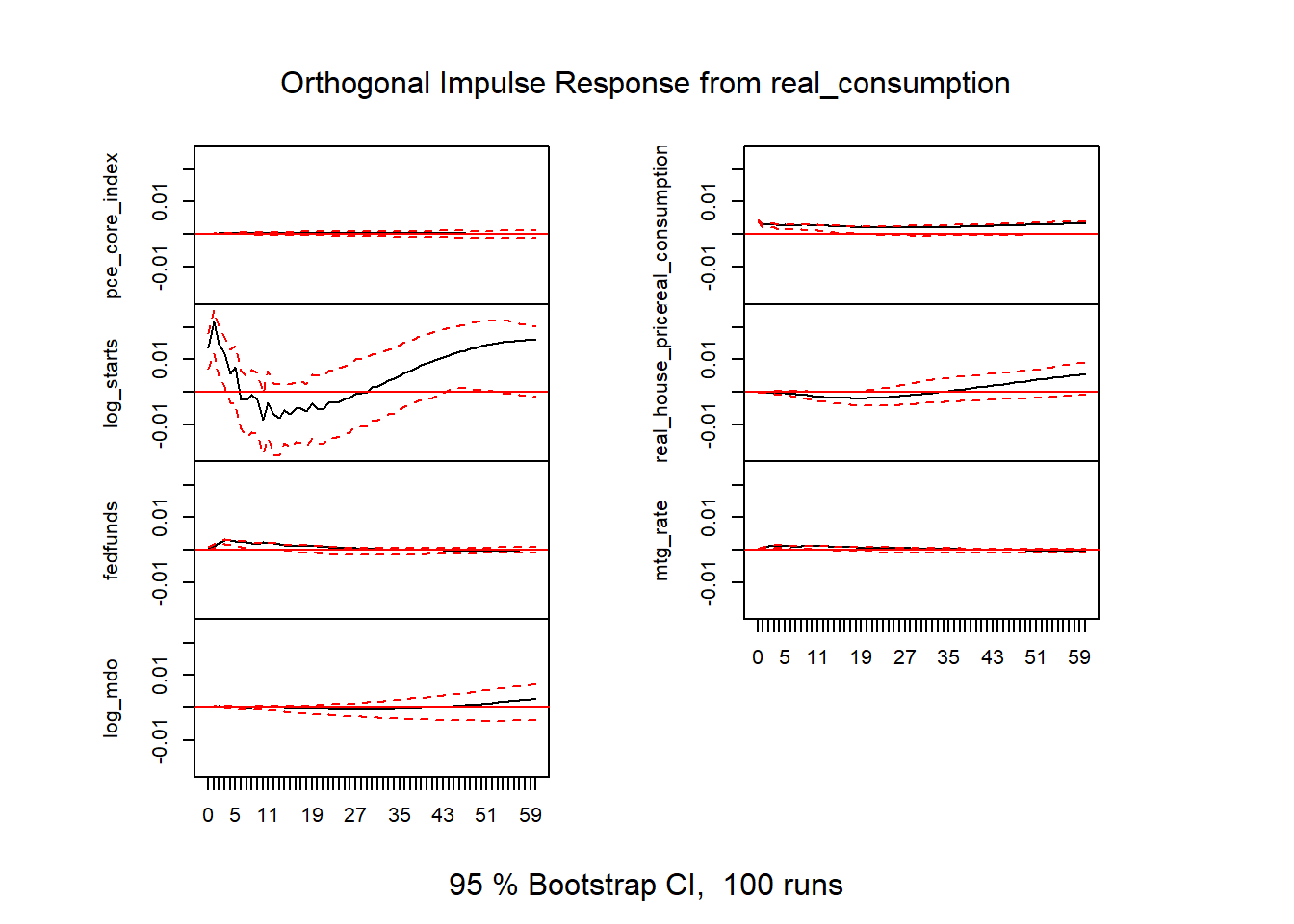
Figure 16: VAR results v2
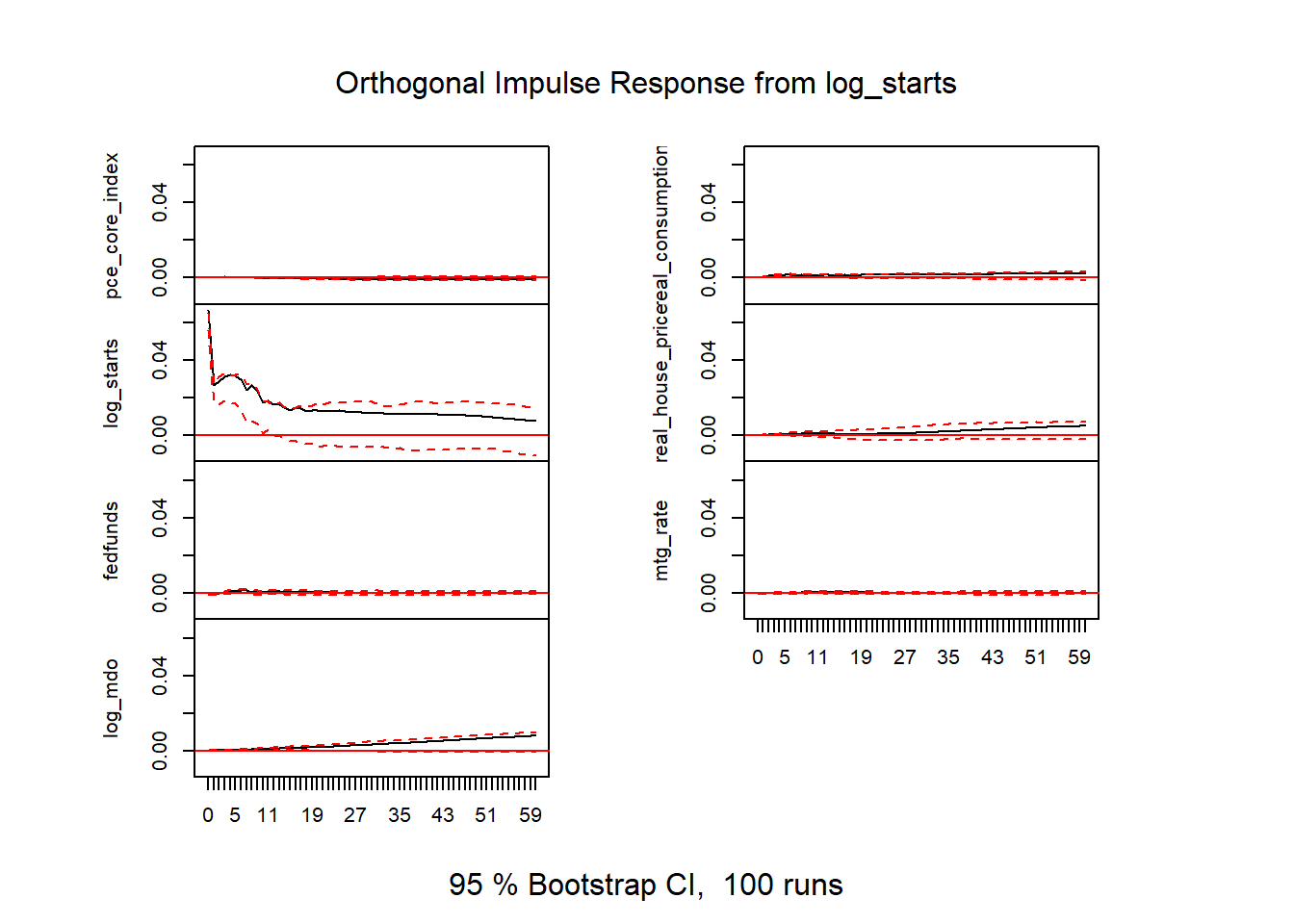
Figure 17: VAR results v2
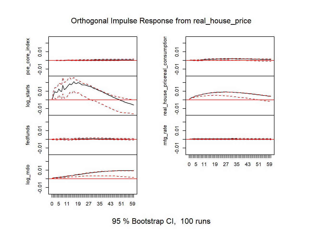
Figure 18: VAR results v2
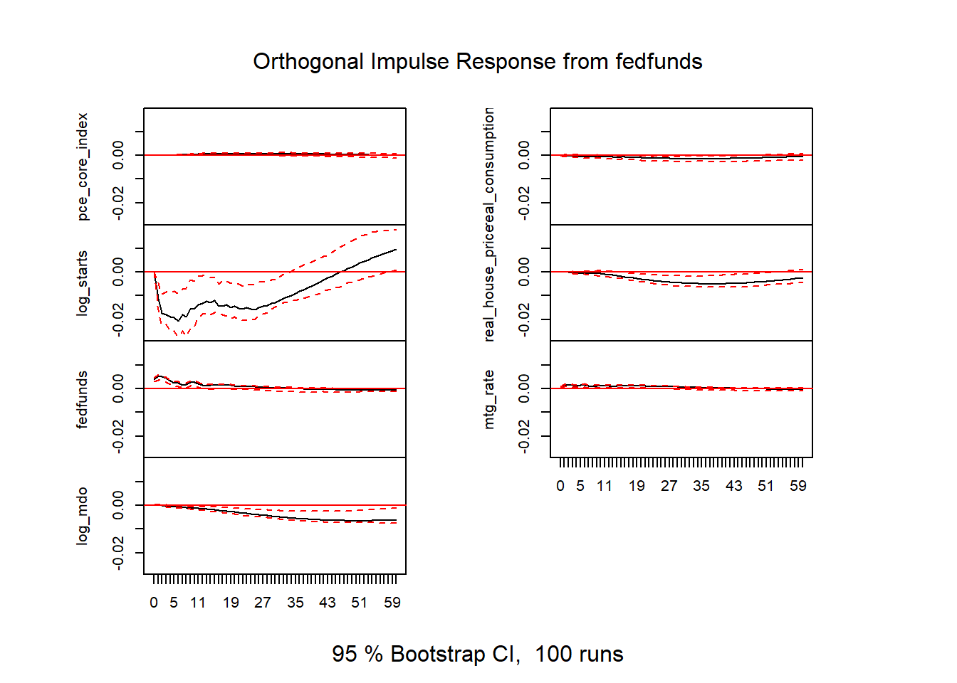
Figure 19: VAR results v2
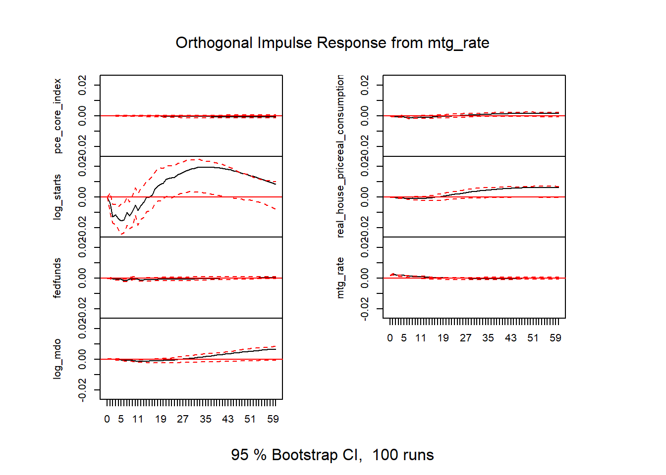
Figure 20: VAR results v2
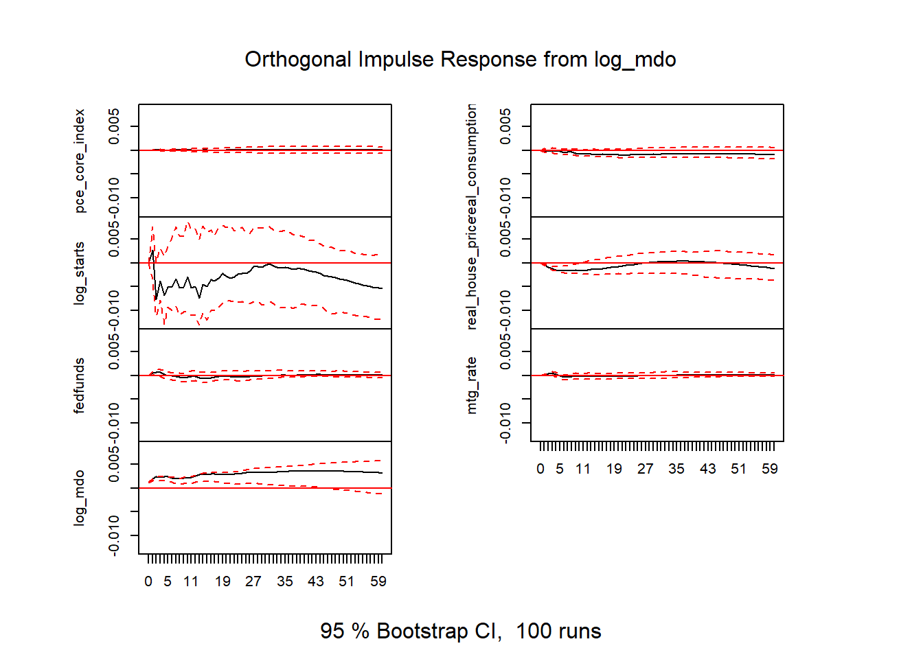
Figure 21: VAR results v2
# response of starts to fed funds
irf_var2_ff_starts <- data.frame(period=1:61,
                       low=irf6$Lower[[5]][,3],
                       up=irf6$Upper[[5]][,3],
                       m = irf6$irf[[5]][,3]
                       )

# response of real house prices to fed funds
irf_var2_ff_rhpi <- data.frame(period=1:61,
                       low=irf6$Lower[[5]][,4],
                       up=irf6$Upper[[5]][,4],
                       m = irf6$irf[[5]][,4]
                       )

# response of mortgage debt outstanding to fed funds
irf_var2_ff_mdo <- data.frame(period=1:61,
                       low=irf6$Lower[[5]][,7],
                       up=irf6$Upper[[5]][,7],
                       m = irf6$irf[[5]][,7]
                       )

# response of log real house prices to log starts
irf_var2_rhpi_starts <- data.frame(period=1:61,
                       low=irf6$Lower[[3]][,4],
                       up=irf6$Upper[[3]][,4],
                       m = irf6$irf[[3]][,4]
                       )

# response of log starts to log real house price
irf_var2_starts_rhpi <- data.frame(period=1:61,
                       low=irf6$Lower[[4]][,3],
                       up=irf6$Upper[[4]][,3],
                       m = irf6$irf[[4]][,3]
                       )

irf_plot3<-
  ggplot(data=irf_var2_ff_starts , aes(x=period,y=m,ymin=low,ymax=up))+
  geom_ribbon(fill="dodgerblue",alpha=0.5)+
  geom_line(color="red")+
  geom_hline(yintercept=0,linetype=2)+
  theme(plot.caption=element_text(hjust=0))+
  scale_y_continuous(labels=scales::percent)+
  scale_x_continuous(breaks=seq(0,60,12))+
  labs(x="months since shock",
       y="Response of log starts (% change in starts)",
       title="Housing Starts Response to fed funds rate shock",
       subtitle="Red line response, blue shaded area 95% confidence interval",
       caption=paste0("@lenkiefer Response estimated by VAR. Response of LOG_STARTS to 1 s.d. fed funds shock",
                      "\nusing R pacake vars: https://CRAN.R-project.org/package=vars",
                      "\nResponse is based on seven variable system with loge core PCE price index, log real consumption expenditures",
                      "\nlog real house price index, log housing starts the 10-year the effective federal funds rate",
                      "\n the 30-year fixed mortgage rate and the log of mortgage debt outstanding",
                      "\nMonthly data Jan 1975 to Sep 2019",
                      "\nSources: Census/HUD,BEA, Federal Reserve, Freddie Mac",
                      "\nRetrieved from FRED, Federal Reserve Bank of St. Louis"))


irf_plot4<-
  ggplot(data=irf_var2_ff_rhpi , aes(x=period,y=m,ymin=low,ymax=up))+
  geom_ribbon(fill="dodgerblue",alpha=0.5)+
  geom_line(color="red")+
  geom_hline(yintercept=0,linetype=2)+
  theme(plot.caption=element_text(hjust=0))+
  scale_y_continuous(labels=scales::percent)+
  scale_x_continuous(breaks=seq(0,60,12))+
  labs(x="months since shock",
       y="Response of log real house price index",
       title="Real house price index response to fed funds rate shock",
       subtitle="Red line response, blue shaded area 95% confidence interval",
       caption=paste0("@lenkiefer Response estimated by VAR. Response of log real house price index to 1 s.d. fed funds shock",
                      "\nusing R pacake vars: https://CRAN.R-project.org/package=vars",
                      "\nResponse is based on seven variable system with loge core PCE price index, log real consumption expenditures",
                      "\nlog real house price index, log housing starts the 10-year the effective federal funds rate",
                      "\n the 30-year fixed mortgage rate and the log of mortgage debt outstanding",
                      "\nMonthly data Jan 1975 to Sep 2019",
                      "\nSources: Census/HUD,BEA, Federal Reserve, Freddie Mac",
                      "\nRetrieved from FRED, Federal Reserve Bank of St. Louis"))

irf_plot5<-
  ggplot(data=irf_var2_ff_mdo , aes(x=period,y=m,ymin=low,ymax=up))+
  geom_ribbon(fill="dodgerblue",alpha=0.5)+
  geom_line(color="red")+
  geom_hline(yintercept=0,linetype=2)+
  theme(plot.caption=element_text(hjust=0))+
  scale_y_continuous(labels=scales::percent)+
  scale_x_continuous(breaks=seq(0,60,12))+
  labs(x="months since shock",
       y="Response of log mdo",
       title="Log mortgage debt outstanding response to fed funds rate shock",
       subtitle="Red line response, blue shaded area 95% confidence interval",
       caption=paste0("@lenkiefer Response estimated by VAR. Response of log mortgage debt outstanding to 1 s.d. fed funds shock",
                      "\nusing R pacake vars: https://CRAN.R-project.org/package=vars",
                      "\nResponse is based on seven variable system with loge core PCE price index, log real consumption expenditures",
                      "\nlog real house price index, log housing starts the 10-year the effective federal funds rate",
                      "\n the 30-year fixed mortgage rate and the log of mortgage debt outstanding",
                      "\nMonthly data Jan 1975 to Sep 2019",
                      "\nSources: Census/HUD,BEA, Federal Reserve, Freddie Mac",
                      "\nRetrieved from FRED, Federal Reserve Bank of St. Louis"))


irf_plot6<-
  ggplot(data=irf_var2_rhpi_starts  , aes(x=period,y=m,ymin=low,ymax=up))+
  geom_ribbon(fill="dodgerblue",alpha=0.5)+
  geom_line(color="red")+
  geom_hline(yintercept=0,linetype=2)+
  theme(plot.caption=element_text(hjust=0))+
  scale_y_continuous(labels=scales::percent)+
  scale_x_continuous(breaks=seq(0,60,12))+
  labs(x="months since shock",
       y="Response of real house prices to starts",
       title="Real house price response to housing starts shock",
       subtitle="Red line response, blue shaded area 95% confidence interval",
       caption=paste0("@lenkiefer Response estimated by VAR. Response of real house price index to 1 s.d. log housing starts shock",
                      "\nusing R pacake vars: https://CRAN.R-project.org/package=vars",
                      "\nResponse is based on seven variable system with loge core PCE price index, log real consumption expenditures",
                      "\nlog real house price index, log housing starts the 10-year the effective federal funds rate",
                      "\n the 30-year fixed mortgage rate and the log of mortgage debt outstanding",
                      "\nMonthly data Jan 1975 to Sep 2019",
                      "\nSources: Census/HUD,BEA, Federal Reserve, Freddie Mac",
                      "\nRetrieved from FRED, Federal Reserve Bank of St. Louis"))

irf_plot7<-
  ggplot(data=irf_var2_starts_rhpi , aes(x=period,y=m,ymin=low,ymax=up))+
  geom_ribbon(fill="dodgerblue",alpha=0.5)+
  geom_line(color="red")+
  geom_hline(yintercept=0,linetype=2)+
  theme(plot.caption=element_text(hjust=0))+
  scale_y_continuous(labels=scales::percent)+
  scale_x_continuous(breaks=seq(0,60,12))+
  labs(x="months since shock",
       y="Response of log starts (% change in starts)",
       title="Housing starts response to real house price shock",
       subtitle="Red line response, blue shaded area 95% confidence interval",
       caption=paste0("@lenkiefer Response estimated by VAR. Response of log housing starts to s.d. real house price shock",
                      "\nusing R pacake vars: https://CRAN.R-project.org/package=vars",
                      "\nResponse is based on seven variable system with loge core PCE price index, log real consumption expenditures",
                      "\nlog real house price index, log housing starts the 10-year the effective federal funds rate",
                      "\n the 30-year fixed mortgage rate and the log of mortgage debt outstanding",
                      "\nMonthly data Jan 1975 to Sep 2019",
                      "\nSources: Census/HUD,BEA, Federal Reserve, Freddie Mac",
                      "\nRetrieved from FRED, Federal Reserve Bank of St. Louis"))
First, let’s look at the response of housing starts to a federal funds rate shock:
irf_plot3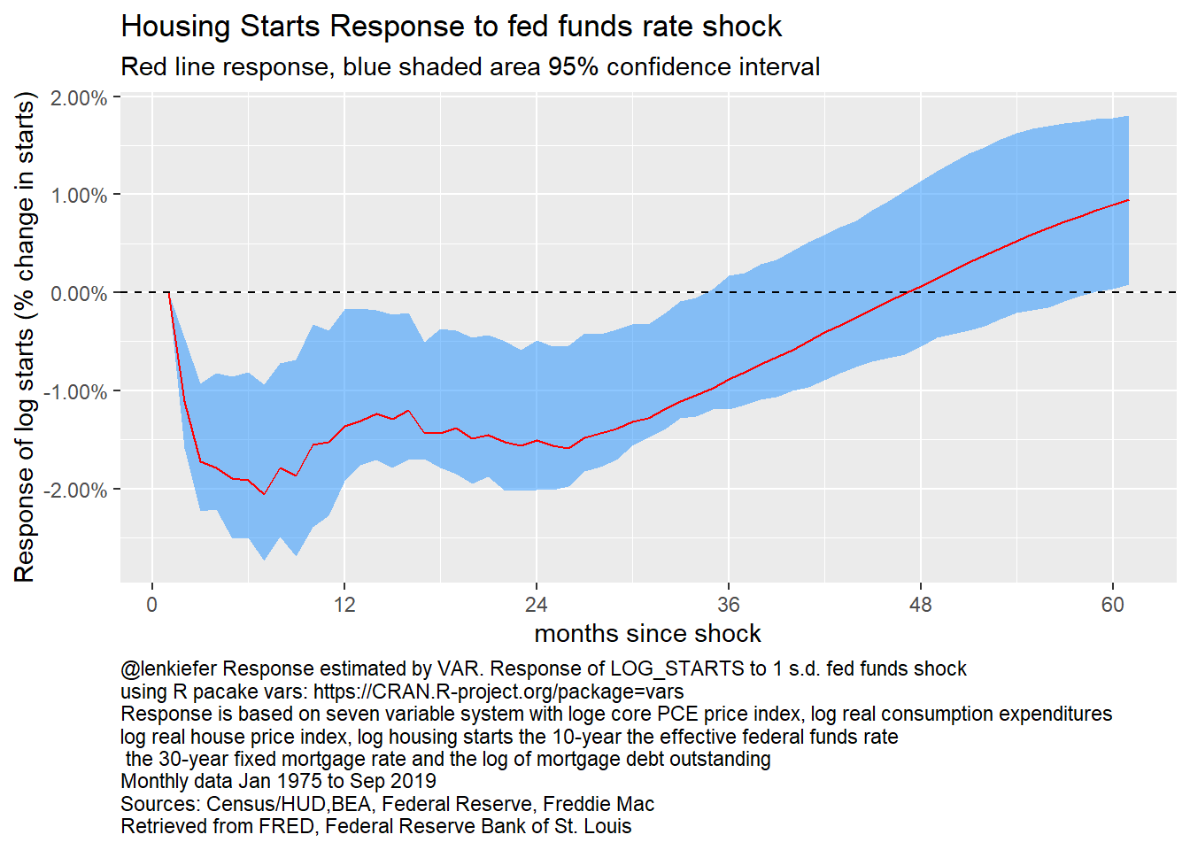
Figure 22: Response of log starts to fed funds rate, 7 variable VAR
Once again, the shock response looks quite similar to the ones above.
It’s also interesting to consider the response of other housing variables. Let’s next look at real house prices.
irf_plot4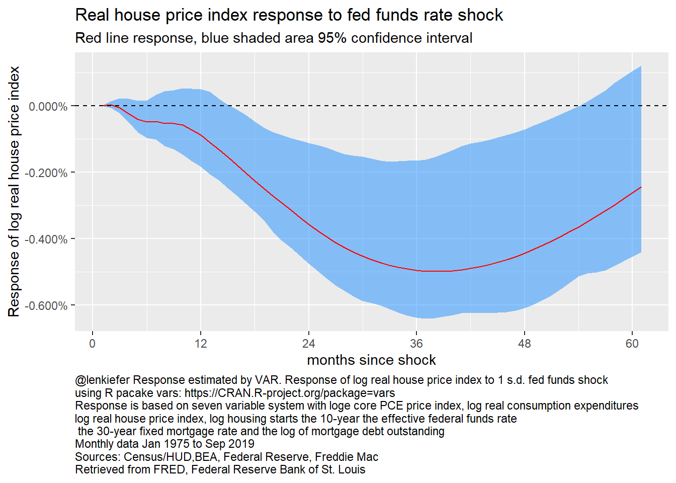
Figure 23: Response of log real house price index to fed funds rate, 7 variable VAR
Following a federal funds rate shock real house prices decline. But the response takes much longer, not reaching a peak decline until almost 3 years after a shock. This reflects the stickiness in real house prices.
How about mortgage debt?
irf_plot5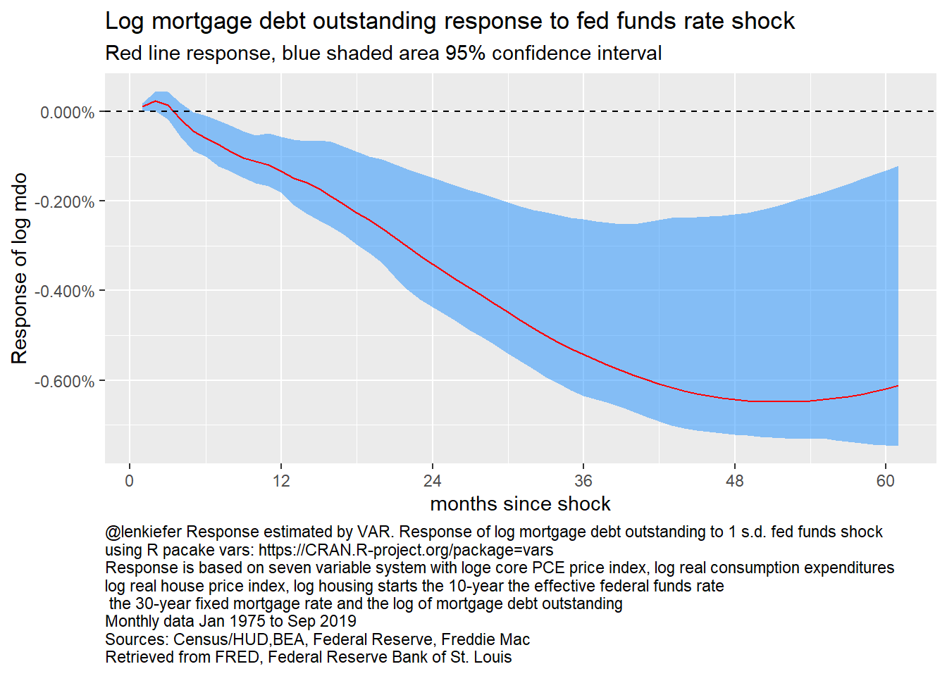
Figure 24: Response of log mortgage debt outstanding to fed funds rate, 7 variable VAR
Following a rate shock, mortgage debt outstanding contracts. After 4 years mortgage debt outstanding declines about 0.8 percentage points.
We can also consider the response of housing to other types of shocks.
Let’s see how real house prices respond to an investment shock (housing starts).
irf_plot6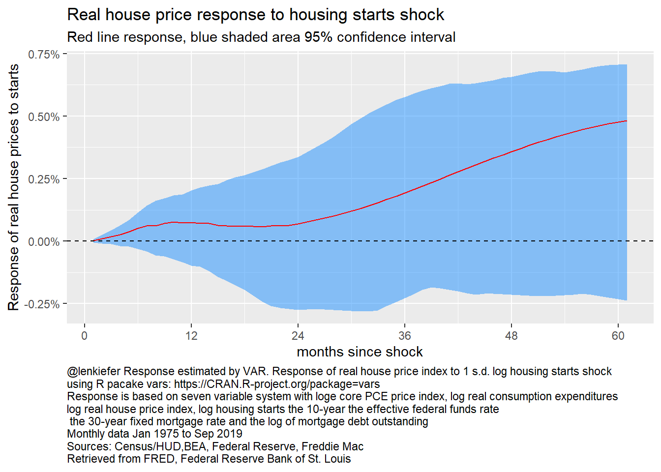
Figure 25: Reponse of log real house prices to log housing starts, 7 variable VAR
House prices again have a delayed reaction. They increase, though the confidence bands include zero throughout.
While real house prices are not responsive to investment, we can see how investment responds to prices in the next plot.
irf_plot7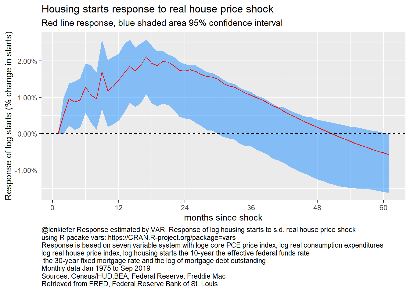
Figure 26: Response of log housing starts to log real house prices, 7 variable VAR
A positive shock to real house prices leads to a sustained increase in housing starts, peaking at about 2 percent around a year and a half following a real house price shock.
Summary and discussion
In this post we covered a lot of ground. We estimated 4 models
- A 5 variable VAR Jan 1960-Sep 2019 with recursive identification
- A 5 variable system, estimated by local projections (Jan 1960 - Sep 2019)
- The same 5 variable system, but this time with responses identified by sign restrictions
- A 7 variable system Jan 1975-Sep 2019
In each model we saw a sustained decline in housing activity following a shock to interest rates. While the results are not conclusive (there are many potential flaws in the identificaton and specification above) they do provide some evidence that following an interest rate increase housing activity contracts.
Since the system is linear, we can invert the relationships. If housing responds negatively to rates increases, according to these models housing responds positvely to decreased rates.
We could consider alternative specification, alternative variables, etc, but we will leave that for future.
References
Fry, R., & Pagan, A. (2011). Sign restrictions in structural vector autoregressions: A critical review. Journal of Economic Literature, 49(4), 938-60. link
Hamilton, J. D. (1994). Time series analysis. Princeton University Press, USA.
Jordà, Ò. (2005). Estimation and inference of impulse responses by local projections. American economic review, 95(1), 161-182.
Lütkepohl, H. (2005). New introduction to multiple time series analysis. Springer Science & Business Media.
Musso, A., Neri, S., & Stracca, L. (2011). Housing, consumption and monetary policy: How different are the US and the euro area?. Journal of Banking & Finance, 35(11), 3019-3041. pdf