It’s been a while since I posted here. I’ve got some longer form things in the works, but let’s ease back into it.
Let’s take a look at the latest Job Openings and Labor Turnover Survey (JOLTS) data via the U.S. Bureau of Labor Statistics. This post is an update of this post. Per usual we will make our graphics with R.
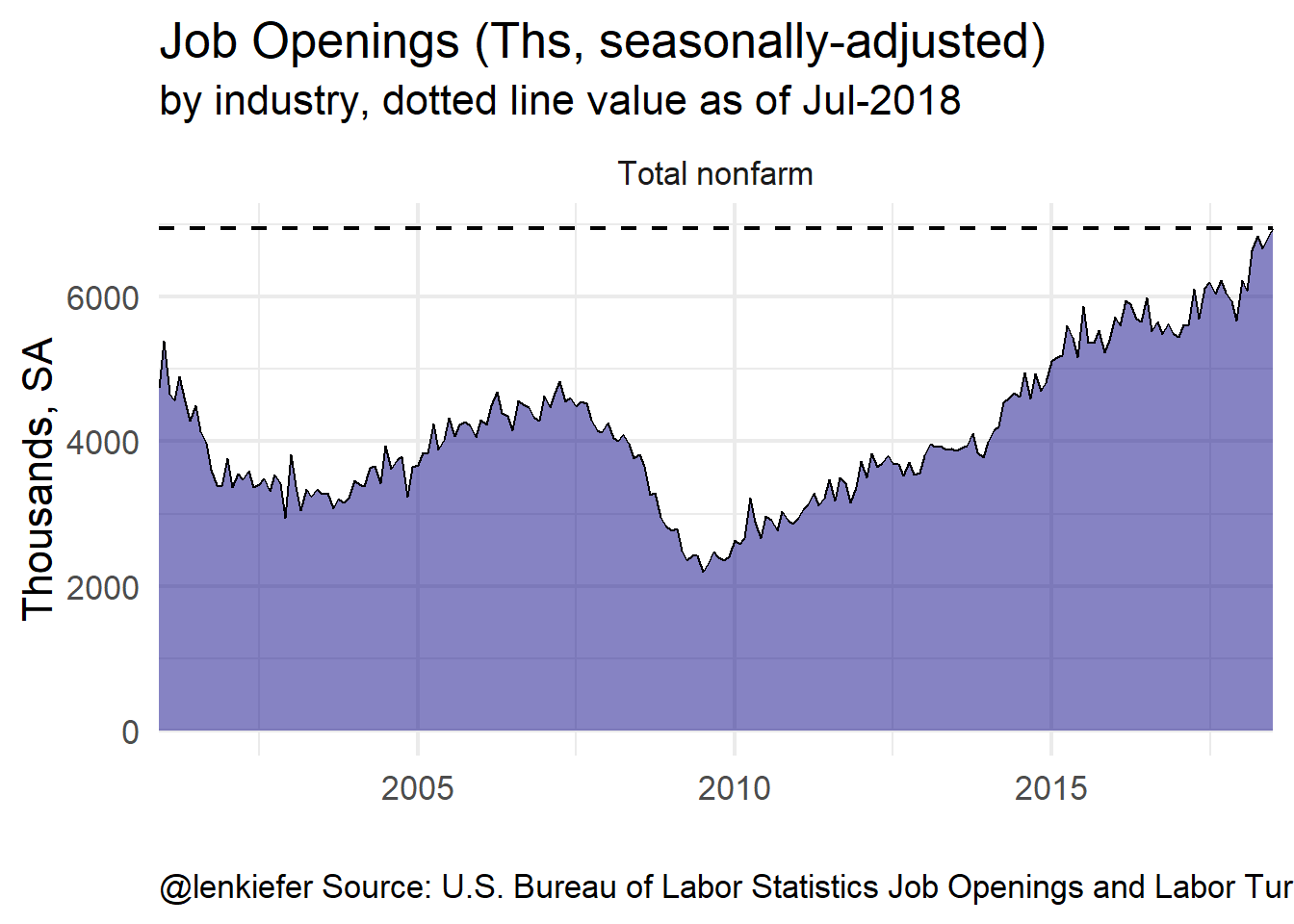
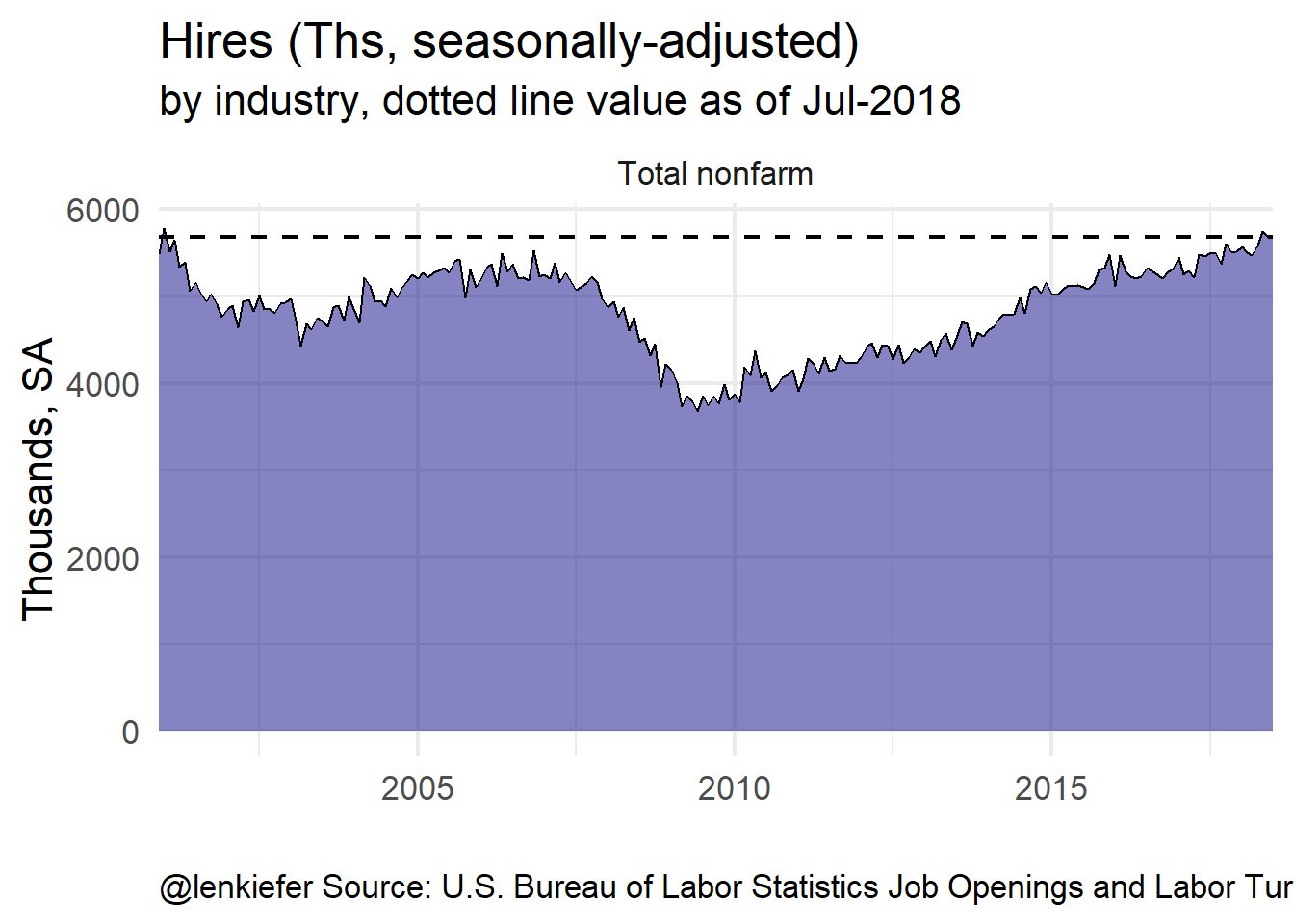
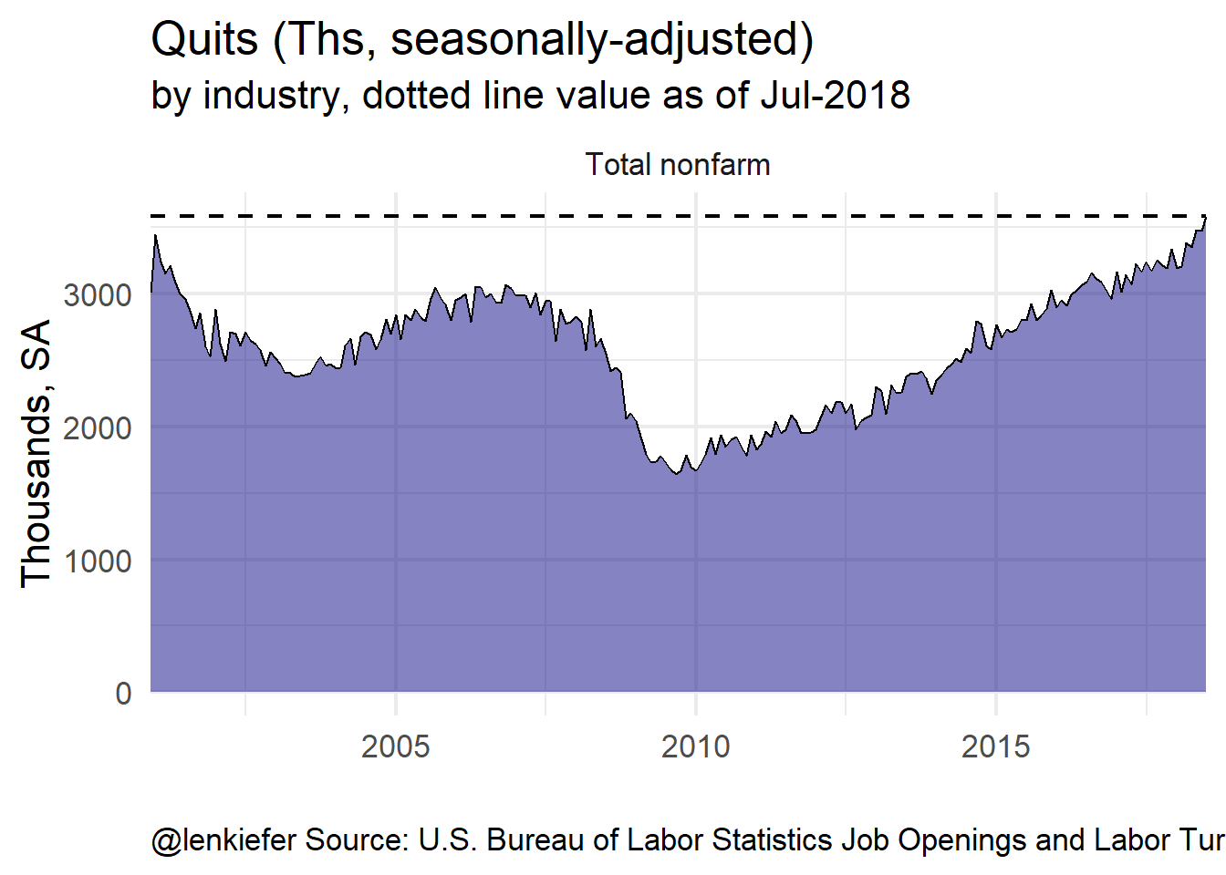
First, let’s look at aggregate trends.
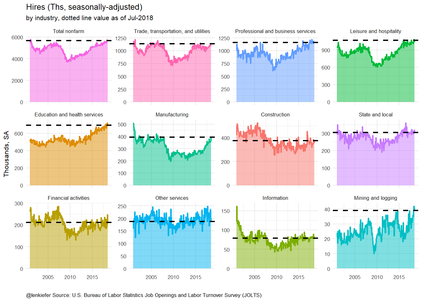
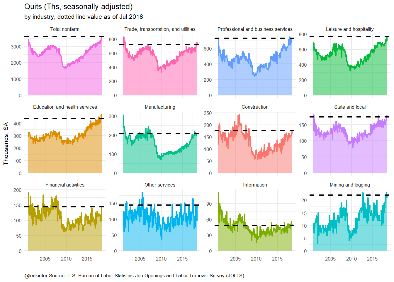
There are a lot of job openings, but hiring has not accelerated. However, as the labor market heats up, more workers are quitting.
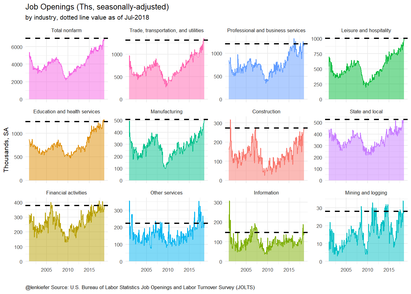
Now let’s look at it by industry.
Panel Plots
R code
We’ve shared similar code before, but for completeness I’ll include it below. After the BLS updated their webpage I was able to update these plots using this code within minutes of the release of the JOLTS data this morning. We just need the tidyverse and data.table libraries to make this work.
Code for Data Wrangling
# load libraries ----
library(data.table)
library(tidyverse)

# get data ---
jolts.dt<-fread("http://download.bls.gov/pub/time.series/jt/jt.data.1.AllItems")
jolts.series<-fread("http://download.bls.gov/pub/time.series/jt/jt.series")
jolts.ind<-fread("http://download.bls.gov/pub/time.series/jt/jt.industry",
                 col.names=c("industry_code","industry_text",   "display_level",    "selectable","sort_sequence"))
jolts.element<-fread("http://download.bls.gov/pub/time.series/jt/jt.dataelement",
                     col.names=c("dataelement_code","dataelement_text","display_level","selectable","sort_sequence","blank"                     ))

#ratelevel: R=rate, L=level
#dataelement_code   dataelement_text    display_level   selectable  sort_sequence
#HI Hires   0   T   2
#JO Job openings    0   T   1
#LD Layoffs and discharges  1   T   5
#OS Other separations   1   T   6
#QU Quits   1   T   4
#TS Total separations   0   T   3

#region_code    region_text display_level   selectable  sort_sequence
#00 Total US    0   T   1
#MW Midwest (Only available for Total Nonfarm)  1   T   4
#NE Northeast (Only available for Total Nonfarm)    1   T   2
#SO South (Only available for Total Nonfarm)    1   T   3
#WE West (Only available for Total Nonfarm) 1   T   5

#industries
ind.list<-unique(jolts.series$industry_code)
ind.list1<-unique(jolts.ind[display_level==1,]$industry_code)
ind.list2<-unique(jolts.ind[display_level==2,]$industry_code)
ind.list3<-unique(jolts.ind[display_level==3,]$industry_code)
reg.list<-unique(jolts.series$region_code)
elem.list<-unique(jolts.element$dataelement_code)
#get data

jolts.series[seasonal=="S" & dataelement_code=="HI" &
               ratelevel_code=="R" & region_code=="00", ]

my.series<-jolts.series[seasonal=="S"  &
                          ratelevel_code=="L" & region_code=="00", ]

my.out<-jolts.dt[ series_id %in% my.series$series_id,]
my.out<-merge(my.out,jolts.series[,list(series_id,industry_code,dataelement_code)],by="series_id")
my.out<-merge(my.out,jolts.ind[,list(industry_code,industry_text)],by="industry_code")
my.out[,month:=as.numeric(substr(period,2,3))]
my.out[,date:= as.Date(ISOdate(year,month,1))]

bdata<-my.out[year==2000 & month==12,]
bdata<-dplyr::rename(bdata, value00=value)
bdata<-bdata[, c('value00','series_id'), with = FALSE]
my.out<-merge(my.out,bdata,by="series_id")
my.out[,val00:=100*value/value00]
bdata<-my.out[year==2007 & month==12,]
bdata<-dplyr::rename(bdata, value07=value)
bdata<-bdata[, c('value07','series_id'), with = FALSE]
my.out<-merge(my.out,bdata,by="series_id")
my.out[,val07:=100*value/value07]
my.out<-my.out[order(date,-value00),]
my.out[,industry_textf:=factor(industry_text,levels=unique(my.out$industry_text))]

#levels(my.out$industry_textf)

d.list<-unique(my.out$date)
d.list2<-unique(my.out[date>="2007-12-01",]$date)
N<-length(d.list2)
i <- N
Code for plots
# individual plots----

ggplot(data=my.out[(industry_code==00000 ) &
                     dataelement_code=="JO",],
       aes(x=date,y=value,color=industry_text))+
  facet_wrap(~industry_textf,scales="free_y")+
  scale_fill_viridis_d(option="C")+
  scale_color_viridis_d(option="B")+
  geom_line(data=my.out[(industry_code==00000  )&
                          dataelement_code=="JO",],color=NA)+
  geom_ribbon(alpha=0.5,aes(ymin=0,ymax=value,fill=industry_text),color=NA)+
  geom_line(size=0.5)+
  theme_minimal(base_size=16)+theme(legend.position="none")+
  geom_hline(data=my.out[(industry_code==00000  )&
                           date==d.list2[N] & dataelement_code=="JO",],
             aes(yintercept=value),linetype=2,color="black",size=0.75)+
  scale_x_date(limits=c(min(d.list),max(d.list2)), expand=c(0,0))+
  theme(plot.caption=element_text(hjust=0))+
  labs(x="", y="Thousands, SA",
       subtitle=paste("by industry, dotted line value as of",
                      as.character(d.list2[i],format="%b-%Y")),
       title="Job Openings (Ths, seasonally-adjusted)",
       caption="@lenkiefer Source: U.S. Bureau of Labor Statistics Job Openings and Labor Turnover Survey (JOLTS)")


ggplot(data=my.out[(industry_code==00000 ) &
                     dataelement_code=="HI",],
       aes(x=date,y=value,color=industry_text))+
  facet_wrap(~industry_textf,scales="free_y")+
  scale_fill_viridis_d(option="C")+
  scale_color_viridis_d(option="B")+
  geom_line(data=my.out[(industry_code==00000  )&
                          dataelement_code=="HI",],color=NA)+
  geom_ribbon(alpha=0.5,aes(ymin=0,ymax=value,fill=industry_text),color=NA)+
  geom_line(size=0.5)+
  theme_minimal(base_size=16)+theme(legend.position="none")+
  geom_hline(data=my.out[(industry_code==00000  )&
                           date==d.list2[N] & dataelement_code=="HI",],
             aes(yintercept=value),linetype=2,color="black",size=0.75)+
  scale_x_date(limits=c(min(d.list),max(d.list2)), expand=c(0,0))+
  theme(plot.caption=element_text(hjust=0))+
  labs(x="", y="Thousands, SA",
       subtitle=paste("by industry, dotted line value as of",
                      as.character(d.list2[i],format="%b-%Y")),
       title="Hires (Ths, seasonally-adjusted)",
       caption="@lenkiefer Source: U.S. Bureau of Labor Statistics Job Openings and Labor Turnover Survey (JOLTS)")


ggplot(data=my.out[(industry_code==00000 ) &
                     dataelement_code=="QU",],
       aes(x=date,y=value,color=industry_text))+
  facet_wrap(~industry_textf,scales="free_y")+
  scale_fill_viridis_d(option="C")+
  scale_color_viridis_d(option="B")+
  geom_line(data=my.out[(industry_code==00000  )&
                          dataelement_code=="QU",],color=NA)+
  geom_ribbon(alpha=0.5,aes(ymin=0,ymax=value,fill=industry_text),color=NA)+
  geom_line(size=0.5)+
  theme_minimal(base_size=16)+theme(legend.position="none")+
  geom_hline(data=my.out[(industry_code==00000  )&
                           date==d.list2[N] & dataelement_code=="QU",],
             aes(yintercept=value),linetype=2,color="black",size=0.75)+
  scale_x_date(limits=c(min(d.list),max(d.list2)), expand=c(0,0))+
  theme(plot.caption=element_text(hjust=0))+
  labs(x="", y="Thousands, SA",
       subtitle=paste("by industry, dotted line value as of",
                      as.character(d.list2[i],format="%b-%Y")),
       title="Quits (Ths, seasonally-adjusted)",
       caption="@lenkiefer Source: U.S. Bureau of Labor Statistics Job Openings and Labor Turnover Survey (JOLTS)")


# panel plots ----

myplotf<-function(i=N){
  g<-
    ggplot(data=my.out[(industry_code==00000 |(industry_code !=910000 &
                                                 industry_code %in% ind.list2) )&
                         date<=d.list2[i] &
                         dataelement_code=="JO",],
           aes(x=date,y=value,color=industry_text))+
    facet_wrap(~industry_textf,scales="free_y")+
    geom_line(data=my.out[(industry_code==00000 |(industry_code !=910000 &
                                                    industry_code %in% ind.list2) )&
                            dataelement_code=="JO",],color=NA)+
    geom_ribbon(alpha=0.5,aes(ymin=0,ymax=value,fill=industry_text),color=NA)+
    geom_line(size=0.5)+
    theme_minimal(base_size=8)+theme(legend.position="none")+
    geom_hline(data=my.out[(industry_code==00000 |(industry_code !=910000 & industry_code %in% ind.list2) )&                            date==d.list2[i] & dataelement_code=="JO",],
               aes(yintercept=value),linetype=2,color="black",size=0.75)+
    scale_x_date(limits=c(min(d.list),max(d.list2)))+
    theme(plot.caption=element_text(hjust=0))+
    labs(x="", y="Thousands, SA",
         subtitle=paste("by industry, dotted line value as of",
                        as.character(d.list2[i],format="%b-%Y")),
         title="Job Openings (Ths, seasonally-adjusted)",
         caption="@lenkiefer Source: U.S. Bureau of Labor Statistics Job Openings and Labor Turnover Survey (JOLTS)")
}

myplotf2<-function(i=N){
  g<-
    ggplot(data=my.out[(industry_code==00000 |(industry_code !=910000 &
                                                 industry_code %in% ind.list2) )&
                         date<=d.list2[i] & dataelement_code=="HI",],
           aes(x=date,y=value,color=industry_text))+
    facet_wrap(~industry_textf,scales="free_y")+
    geom_line(data=my.out[(industry_code==00000 |(industry_code !=910000 &
                                                    industry_code %in% ind.list2) )&
                            dataelement_code=="HI",],color=NA)+
    geom_ribbon(alpha=0.5,aes(ymin=0,ymax=value,fill=industry_text),color=NA)+
    geom_line(size=0.85)+
    theme_minimal(base_size=8)+theme(legend.position="none")+
    geom_hline(data=my.out[(industry_code==00000 |(industry_code !=910000 & industry_code %in% ind.list2) )&
                             date==d.list2[i] & dataelement_code=="HI",],
               aes(yintercept=value),linetype=2,color="black",size=0.75)+
    scale_x_date(limits=c(min(d.list),max(d.list2)))+
    theme(plot.caption=element_text(hjust=0))+
    #scale_y_log10()+
    labs(x="", y="Thousands, SA",
         subtitle=paste("by industry, dotted line value as of",
                        as.character(d.list2[i],format="%b-%Y")),
         title="Hires (Ths, seasonally-adjusted)",
         caption="@lenkiefer Source: U.S. Bureau of Labor Statistics Job Openings and Labor Turnover Survey (JOLTS)")
}

myplotf3<-function(i=N){
  ggplot(data=my.out[(industry_code==00000 |(industry_code !=910000 &
                                               industry_code %in% ind.list2) )&
                       date<=d.list2[i] & dataelement_code=="QU",],
         aes(x=date,y=value,color=industry_text))+
    facet_wrap(~industry_textf,scales="free_y")+
    geom_line(data=my.out[(industry_code==00000 |(industry_code !=910000 & industry_code %in% ind.list2) )&
                            dataelement_code=="QU",],color=NA)+

    #scale_y_continuous(limits=c(25,150),breaks=seq(25,175,25))+
    #scale_y_continuous(limits=c(0,250),breaks=seq(0,350,50))+
    geom_ribbon(alpha=0.5,aes(ymin=0,ymax=value,fill=industry_text),color=NA)+
    geom_line(size=0.85)+
    theme_minimal(base_size=8)+theme(legend.position="none")+
    geom_hline(data=my.out[(industry_code==00000 |(industry_code !=910000 & industry_code %in% ind.list2) )&
                             date==d.list2[i] & dataelement_code=="QU",],
               aes(yintercept=value),linetype=2,color="black",size=0.75)+
    scale_x_date(limits=c(min(d.list),max(d.list2)))+
    theme(plot.caption=element_text(hjust=0))+
    #scale_y_log10()+
    labs(x="", y="Thousands, SA",
         subtitle=paste("by industry, dotted line value as of",
                        as.character(d.list2[i],format="%b-%Y")),
         title="Quits (Ths, seasonally-adjusted)",
         caption="@lenkiefer Source: U.S. Bureau of Labor Statistics Job Openings and Labor Turnover Survey (JOLTS)")
}