As an economist with a background in econometrics and forecasting I recognize that predictions are often (usually?) an exercise in futility. Forecasting, after all, is hard. While non-economists have great fun pointing this futility out, many critics miss out on why it’s so hard.
There are at least two reasons why forecasting is hard. The first, the unknown future, is pretty well understood. Empirical regularities with much forecasting power in the social sciences are hard to come by and are rarely stable. Until we develop prehistory or precognition, there is an irreducible uncertainty about the future.
But there’s a second sort of uncertainty. Uncertainty about the present. This uncertainty is in principle reducible. We could go out and learn more about the world, measure more, see more. Statistics and metrics we cover are usually subject to sampling uncertainty and error. I spend a lot of time trying to stitch together bits of information into a composite whole.
One way to do that is the subject of this post. I have been studying a particular kind of problem, and I’m going to share some notes related to that problem. At this point, I’m still puzzling through a few things, so forgive me I appear to wander.
The Filter
About every 18 months or so I have occasion to build or modify a model using the Kalman Filter.The Kalman Filter a useful tool for representing times series data. And each time I come back to it, it seems I’m using different software or different packages. This time, we’re going to use R.
For a full treatment you need a good textbook or a class. I’ve posted some references at the bottom. This post covers usage in R at an introductory level and has some useful links.
A problem
I’m going to focus on a particular example of a statespace model where the filter applies. I’m not going to justify this particular model here, but let’s see how it works. Imagine we wanted to track a time series (say an index of economic activity or a price index), call it \(z_t\). Imagine that \(z_t\) follows an ARIMA(1,1,0) process. Every period (say a month) we observe a noisy signal of the current level of the index \(y_{1,t} = z_{t} + noise\). We also observe a less noisy signal of the level of the index in the prior period \(y_{2,t} = z_{t-1} + noise\) As a good Bayesian we might form a prior expectation of \(z_t\) and then weight the two signals.
How much weight should we put on the two series? If everything is nice and linear and Gaussian (or we were willing to accept that as an approximation), then the Kalman filter will give us the answer. Let’s consider some examples.
As I mentioned, I recode the Kalman Filter about every 18 months or so. The Kalman Filter has a nice recursive representation, so it’s fairly easy to write down. Most packages have a form of built in Kalman Filter (as does R’s stats), but often it isn’t quite flexible for what I need so I just start over. For today I found the dlm package to be useful, but we’ll have to extend it for what I want to do with it. In this post we’ll work through a simple example and see how we can adapt the dlm package along the way.
State process
We need to specify the process. For this example, imagine that our fundamental variable of interest \(z_t\) follows an ARIMA(1,1,0) process with drift. That is:
\[ z_t-z_{t-1} = \mu_z + \rho (z_{t-1}-z_{t-2}) + e_t, e_t \sim N(0,\sigma^{2}_z)\]
Signal process
We also have two signals, one for \(z_t\) and one for \(z_{t-1}\) that we recieve concurrently. Imagine that the signal \(y_{2,t}\) for \(z_{t-1}\) is much more precise but is only available with a lag. The concurrent signal \(y_{1t}\) is noisier and possibly subject to some bias \(\mu_{y1}\).
\[ y_{1,t} = \mu_{y1} + z_{t} + u_{1,t}, u_{1,t} \sim N(0,\sigma^{2}_{u1})\] \[ y_{2,t} = z_{t-1} + u_{2,t}, u_{2,t} \sim N(0,\sigma^{2}_{u2})\] And \(\sigma^{2}_{u1} > \sigma^{2}_{u2}\), perhaps much more so.
Combining into State Space
Part of the fun of working with the Kalman Filter is that it’s ubiquitous and has spread across multiple disciplines so the notation is often slightly different. As we’re going to use the dlm package, we’ll adapt the notation as used in it’s vignette. As I was testing this post I kept getting weird results and only finally realized that the use of \(F\) and \(G\) in the matrix notation was switched between the dlm package and one of my references (Lütkepohl 2005). I also had to go back and edit this post a couple times.
Check one of the references for a general treatment but for our specific problem this will do:
\[ \begin{cases} Z_t = G Z_{t-1} + v_t, v_t \sim N(0,W_t) \\ Y_t = F Z_t + w_t, w_t \sim N(0,V_t)\end{cases}\] Where \(Z_t = \begin{bmatrix} z_t, & z_{t-1},& 1\end{bmatrix}^T\) and
\[ G = \begin{bmatrix} 1+\rho & -\rho & \mu_z\\ 1 & 0 & 0 \\ 0 & 0 & 1\end{bmatrix} \]
And
\[ W_t = \begin{bmatrix} \sigma^{2}_z & 0 & 0\\ 0 & 0 & 0 \\ 0 & 0 & 0\end{bmatrix} \]
Note that the only source of variance in the state vector is in the first row. The lag and constant are carried around in the state vector.
Also,
\[ F = \begin{bmatrix} 1 & 0 & \mu_{y1}\\ 0 & 1 & 0 \\ 0 & 0 & 1\end{bmatrix} \]
And
\[ V_t = \begin{bmatrix} \sigma^{2}_{u1} & 0 & 0\\ 0 & \sigma^{2}_{u2} & 0 \\ 0 & 0 & 0\end{bmatrix} \]
Note that the constant is observed without error.
Simulate the series with R
We can simulate this model using R and the dlm package.
# Load Libraries ----
library(dlm)
library(tidyverse) # for plotting


# set parameters
mu_z <- 0.1
mu_y <- 0.5 # spread between observation and data
rho1 <- 0.9
sig_z <- 1
sig_u1 <- 10
sig_u2 <- 0.1

GG <- matrix(c(1+rho1,-rho1,mu_z,1,0,0,0,0,1),nrow=3,byrow=TRUE)
FF <- matrix(c(1,0,mu_y,0,1,0,0,0,1),nrow=3,byrow=TRUE)
m0 <- matrix(c(0,0,0), nrow=3)
C0 <- matrix(rep(0,9),nrow=3)
W <- matrix(c(sig_z,0,0,
              0,0,0,
              0,0,0),nrow=3,byrow=TRUE)
V <- matrix(c(sig_u1,0,0,
              0,sig_u2,0,
              0,0,0),nrow=3,byrow=TRUE)
my_dlm <- dlm(FF=FF,V=V,GG=GG,W=W,V=V,m0=c(0,0,1),C0=C0)
After setting it up we can simulate from the process using dlm::dlmForecast.
set.seed(20180610)  #set seed for reproducible results
y1 <- dlmForecast(my_dlm, nAhead=120,sampleNew=1)
df <- data.frame(y=y1$newObs, z=y1$newStates)
df$id <- seq.int(nrow(df))
ggplot(data=df, aes(x=id,y=y.1))+
  geom_line()+
  geom_line(linetype=2,aes(y=z.1),color="red")+
  labs(x="time",y="Z", title="Simulated dynamic linear model", subtitle="black solid line observation y1\nred dotted line fundamental z")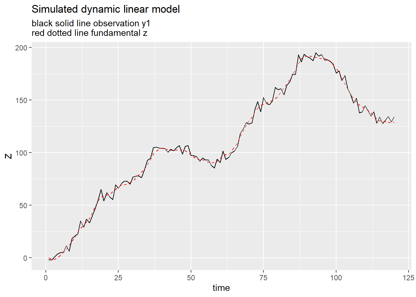
Estimating DLM
The dlm package allows you to estimate a dlm model using Maximum Likelihood. Let’s check using the simulated series. If we simulate our series and then estimate the process using only the simulated signals, do we get back something reasonable close to the original process?
my_dlmfc <- function(par=c(rho1,sig_z,sig_u1,sig_u2,mu_z,mu_y)){
  rho1 = par[1]
  sig_z = par[2]
  sig_u1 = par[3]
  sig_u2 = par[4]
  mu_z = par[5]
  mu_y = par[6]
  GG <- matrix(c(1+rho1,-rho1,mu_z,1,0,0,0,0,1),nrow=3,byrow=TRUE)
  FF <- matrix(c(1,0,mu_y,0,1,0,0,0,1),nrow=3,byrow=TRUE)
  m0 <- matrix(c(0,0,0), nrow=3)
  C0 <- matrix(rep(0,9),nrow=3)
  W <- matrix(c(sig_z,0,0,
                0,0,0,
                0,0,0),nrow=3,byrow=TRUE)
  V <- matrix(c(sig_u1,0,0,
                0,sig_u2,0,
                0,0,0),nrow=3,byrow=TRUE)
  my_dlm3 <- dlm(FF=FF,V=V,GG=GG,W=W,V=V,m0=c(0,0,1),C0=C0)
  return(my_dlm3)
}

my_mle <- dlmMLE(matrix(unlist(y1$newObs),ncol=2),
                 rep(0.5,6),  #set initial values
                 my_dlmfc, lower=c(-1,0,0,0,-Inf,-Inf) # as dlmMLE uses optim L-BFGS-B method by default we can set lower/upper bounds to parameters to keep us out of trouble
                 )
my_comp <- data.frame(row.names=c("rho1","sig_z","sig_u1","sig_u2","mu_z","mu_y"),real=c(rho1,sig_z,sig_u1,sig_u2,mu_z,mu_y), mle=my_mle$par)
knitr::kable(my_comp,digits=3, caption = "Checking MLE against simulated data")| real | mle | |
|---|---|---|
| rho1 | 0.9 | 0.919 |
| sig_z | 1.0 | 1.156 |
| sig_u1 | 10.0 | 13.994 |
| sig_u2 | 0.1 | 0.196 |
| mu_z | 0.1 | 0.085 |
| mu_y | 0.5 | 0.461 |
Okay, looks pretty close to the true process.
I was interested in seeing how variations in the parameters of this model might affect the relative value of the signals. If the concurrent estimate is very noisy, then we might not put much weight on it. In the context of the Kalman Filter the Kalman Gain serves as a useful summary statistic. Unfortunately, the dlm library doesn’t give you back the gain, but it does give you the information you need to construct it. We can write a little function to extract the gain given a dlm model.
my_kgain <- function(i=1, # signal input ( 1 or 2 in our example)
                     j=1, # gain location (should be 1 or 2 in our exmample)
                     j2=1, # should be same as j
                     myk.in=myk,   # input results, the output of a dlmFilter call (see below)
                     my_dlm.in = my_dlm2 # input dlm object, result of dlm call (see below)
                     ){
  vmt <- myk.in$U.C[[i]] %*% diag(myk.in$D.C[i,] ^ 2) %*% t(myk.in$U.C[[i]])
  vat <- myk.in$U.R[[i]] %*% diag(myk.in$D.R[i,] ^ 2) %*% t(myk.in$U.R[[i]])
  K_gain <-vat* t(FF(my_dlm.in)) * solve(FF(my_dlm.in)* vat * t(FF(my_dlm.in)) + V(my_dlm.in))
  return(K_gain[[j,j2]])
}

# estimated gain:
myf <- function(par=c(rho1,sig_z,sig_u1,sig_u2,mu_z,mu_y)){
  rho1 = par[1]
  sig_z = par[2]
  sig_u1 = par[3]
  sig_u2 = par[4]
  mu_z = par[5]
  mu_y = par[6]
  GG <- matrix(c(1+rho1,-rho1,1,0),nrow=2,byrow=TRUE)
  FF <- matrix(c(1,0,0,1),nrow=2,byrow=TRUE)
  m0 <- matrix(c(0,0), nrow=2)
  C0 <- matrix(rep(0,4),nrow=2)
  W <- matrix(c(sig_z,0,0,0),nrow=2,byrow=TRUE)
  V <- matrix(c(sig_u1,0,0,sig_u2),nrow=2,byrow=TRUE)
  my_dlm3 <- dlm(FF=FF,V=V,GG=GG,W=W,V=V,m0=c(0,0),C0=C0)
  y1 <- dlmForecast(my_dlm3, nAhead=20,sampleNew=1)
  df <- data.frame(y=y1$newObs, z=y1$newStates)
  df$id <- seq.int(nrow(df))
  myk <- dlmFilter(as.matrix(df[,1:2]), my_dlm3)
  dfk <- data.frame(id=1:nrow(myk$a)) %>% mutate(k11=map(id,my_kgain,1,1,myk,my_dlm3),
                                                 k12=map(id,my_kgain,1,2,myk,my_dlm3),
                                                 k21=map(id,my_kgain,2,1,myk,my_dlm3),
                                                 k22=map(id,my_kgain,2,2,myk,my_dlm3) )
  return(tail(dfk,1) %>% select(k11,k22))
}
knitr::kable(myf(my_comp$mle)  %>%  unlist %>% t %>% data.frame,
             digits=3,
             row.names=F,
             col.names=c("Gain for y_1","Gain for y_2"),
caption="Kalman Gain After 20 Periods")| Gain for y_1 | Gain for y_2 |
|---|---|
| 0.308 | 0.891 |
Now we can see how the gain varies for different parameterizations. We will fix the innovation variance for the unobserved series so that \(\sigma_z^2=1\) and we’ll set the intercepts \(mu_z\) and \(mu_y\) equal to 0. Setting the intercepts equal to zero allows us to drop one of the state variables. I originally wrote the code without an intercept, and only later added it. I’ve updated the code to carry the intercept around in case you want to add it back.
# estimated gain:
myf2 <- function(rho1 = 0.9 ,
                   sig_z = 1,
                   sig_u1 = 10,
                   sig_u2 = 0.001,
                   mu_z=0,
                   mu_y=0){

 GG <- matrix(c(1+rho1,-rho1,1,0),nrow=2,byrow=TRUE)
  FF <- matrix(c(1,0,0,1),nrow=2,byrow=TRUE)
  m0 <- matrix(c(0,0), nrow=2)
  C0 <- matrix(rep(0,4),nrow=2)
  W <- matrix(c(sig_z,0,0,0),nrow=2,byrow=TRUE)
  V <- matrix(c(sig_u1,0,0,sig_u2),nrow=2,byrow=TRUE)
  my_dlm3 <- dlm(FF=FF,V=V,GG=GG,W=W,V=V,m0=c(0,0),C0=C0)
  y1 <- dlmForecast(my_dlm3, nAhead=20,sampleNew=1)
  df <- data.frame(y=y1$newObs, z=y1$newStates)
  df$id <- seq.int(nrow(df))
  myk <- dlmFilter(as.matrix(df[,1:2]), my_dlm3)
  dfk <- data.frame(id=1:nrow(myk$a)) %>% mutate(k11=map(id,my_kgain,1,1,myk,my_dlm3),
                                                 k12=map(id,my_kgain,1,2,myk,my_dlm3),
                                                 k21=map(id,my_kgain,2,1,myk,my_dlm3),
                                                 k22=map(id,my_kgain,2,2,myk,my_dlm3) )
  return(tail(dfk,1) %>% select(k11,k22))
}


df_test <- expand.grid(r=seq(0,.9,.1), sm=c(0.01,1,10), sp=c(0.01,1,10), mu_z=0,mu_y=0) %>%

  mutate(kgain=as.vector(pmap(list(rho1=r,sig_z=1,sig_u1=sm,sig_u2=sp,mu_z=0,mu_y=0),myf2))) %>%
  unnest(kgain) %>% mutate(k11=unlist(k11,use.names=FALSE),
                           k22=unlist(k22,use.names=FALSE)
                           )
ggplot(data=df_test, aes(x=r, y=k11))+geom_line(size=1.1)+
facet_grid(paste0("Sigma_y1 = ",format(sm,scientific=F))~paste0("Sigma_y2= ",format(sp, scientific=F)))+
labs(x="rho1", y="Kalman Gain For Y1 (T=20)",
title="Gain for Y1",
subtitle="Kalman gain increases with rho (Sigma_z fixed at 1)")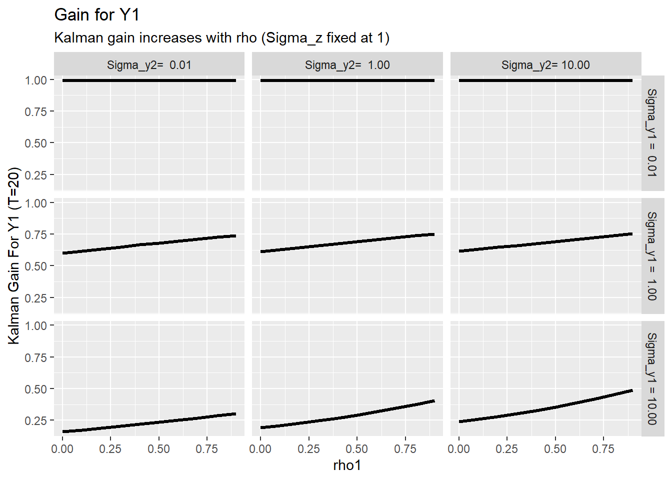
ggplot(data=df_test, aes(x=r, y=k22))+geom_line(size=1.1)+
facet_grid(paste0("Sigma_y1 = ",format(sm,scientific=F))~paste0("Sigma_y2= ",format(sp, scientific=F)))+
labs(x="rho1", y="Kalman Gain For Y2(T=20)",
title="Gain for Y2",
subtitle="Kalman gain increases with rho (Sigma_z fixed at 1)")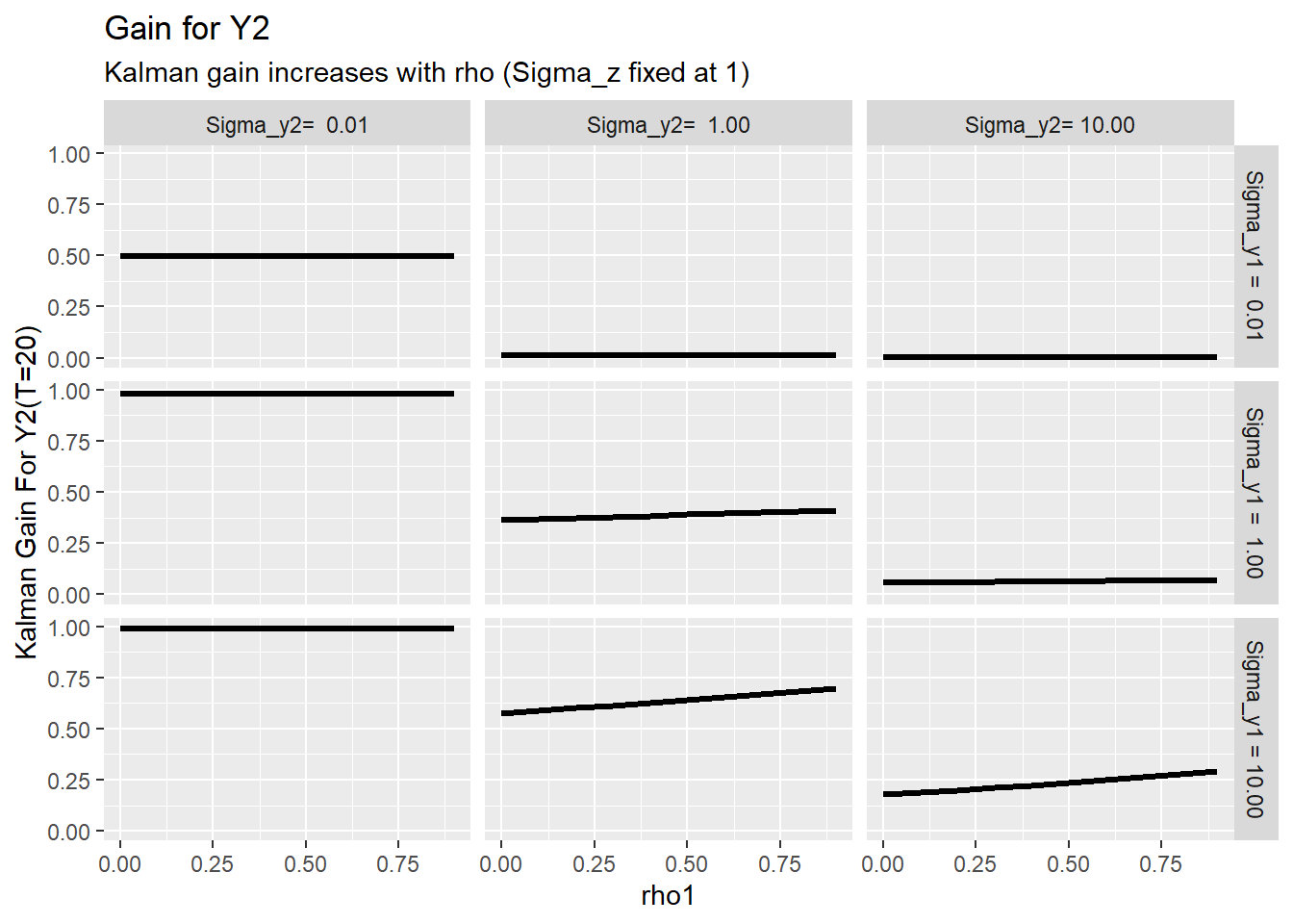 The facets help I think, but we could try to put them all on one plot:
ggplot(data=df_test, aes(x=r, y=k11, color=paste0("Sigma_y2= ",format(sp, scientific=F)), linetype=paste0("Sigma_y1 = ",format(sm,scientific=F))))+geom_path(size=1.1)+
  theme(legend.position="top")+
  scale_linetype(name="sig_u1")+
  scale_color_discrete(name="sig_u2")+
    labs(x="rho1", y="Kalman Gain For Y2(T=20)",
       title="Gain for Y1",
       subtitle="Kalman gain increases with rho (Sigma_z fixed at 1)")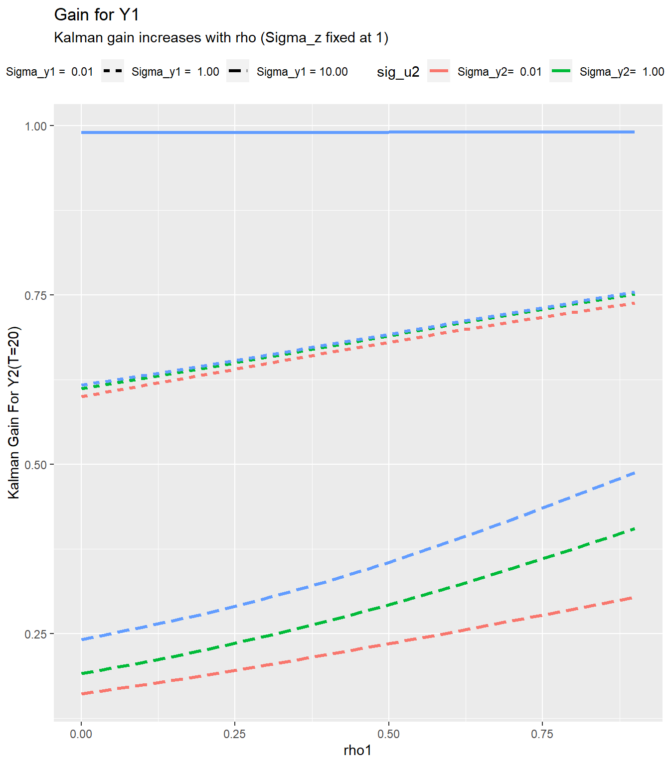
A little discussion
This little analysis shows that as the persistence in the latent time series \(z_t\) increases (\(\rho\) becomes bigger), the value of informaiton as summarized by the Kalman gain increases.
An interesting emprical question then is what are the relative variances of the signals. What sort of time series might follow this kind of process. For that, we’ll need a follow up post.
References
Some useful time series references with details on the Kalman Filter
Giovanni Petris (2010). An R Package for Dynamic Linear Models. Journal of Statistical Software, 36(12), 1-16. URL http://www.jstatsoft.org/v36/i12/.
Hamilton, J. D. (1994). Time series analysis (Vol. 2). Princeton: Princeton university press.
Lütkepohl, H. (2005). New introduction to multiple time series analysis. Springer Science & Business Media.
Petris, Petrone, and Campagnoli. Dynamic Linear Models with R. Springer (2009).
Restored 2021-09-23