I LIKE TO MAKE ANIMATIONS WITH R. Sometimes folks ask me how they add to understanding. They don’t always, but often, particularly when you are working with time series, I find they help visualize trends and understand the evolution of variables.
I’ve written several posts on animation, see particularly this recent post on making a simple line plot and this post about improving animations with tweenr.
Tweenr is a handy package that lets you interpolate data and make smooth animations. The package author Thomas Lin Pedersen homepage [Twitter: @thomasp85](https://twitter.com/thomasp85) tweeted to me that he’s been developing some new functions.
Thomas’s tween indicated that tweenr was now pipe friendly:
Tweenr be pipe-friendly! @lenkiefer, as a certified tween-master can I get your opinion on tween_state() just added to GitHub?
— Thomas Lin Pedersen (@thomasp85) March 16, 2018
Let’s test it out. At least at time of writing, you’ll need to get the development version of tweenr from github in order to recreate all these animations.
Some sample data
For today’s exercise I wanted to make visualizations of house prices. We’ll work with the Federal Housing Finance Agency’s All Transactions House Price Index, which is available quarterly for United States and the 50 states plus the District of Columbia.
We’ll pull the data via the St Louis Federal Reserve Economic Database FRED. See here for more on using the quantmod and tidyquant packages to work with FRED data.
The following data will prepare our data (see how easy it is with tidyquant and the tidyverse).
#####################################################################################
## Step 1: Load Libraries ##
#####################################################################################
library(tidyverse)
library(tidyquant)
library(geofacet)
library(viridis)
library(scales)
library(tweenr)
library(animation)
library(dplyr)

#####################################################################################
## Step 2: go get data ##
## FHFA's ALL-Transactions House Price Index for US and states (NSA) **
#####################################################################################
df <- tq_get(c("USSTHPI",paste0(us_state_grid3$code,      # get state abbreviations
                    "STHPI")),                    # append STHPI
             get="economic.data",             # use FRED
             from="2000-01-01")               # go from 1990 forward

df %>% mutate(state=substr(symbol,1,2)        # create a state variable
) -> df


df %>% group_by(state) %>%
  mutate(hpi=100*price/price[date=="2000-01-01"]) %>% # rebenchmark index to 100 in Q1 2000
    ungroup() %>%
  map_if(is.character,as.factor) %>%   # tweenr will try to interpolate characters, but will ignore factors
  as.tibble() -> df
knitr::kable(head(df))| symbol | date | price | state | hpi |
|---|---|---|---|---|
| USSTHPI | 2000-01-01 | 228.82 | US | 100.0000 |
| USSTHPI | 2000-04-01 | 232.55 | US | 101.6301 |
| USSTHPI | 2000-07-01 | 236.78 | US | 103.4787 |
| USSTHPI | 2000-10-01 | 240.43 | US | 105.0739 |
| USSTHPI | 2001-01-01 | 246.35 | US | 107.6610 |
| USSTHPI | 2001-04-01 | 250.48 | US | 109.4660 |
Now we’ll have a simple data frame with columns corresponding to house prices (original indexed to 1980Q1 =100 and our revised index with 2000 Q1 = 100), state, and date.
Using tween_element
The new pip-friendly tween_element function allows us to pipe in commands, which not only makes our code a little more readable, it also helps you construct an animation piece by piece.
Consider this spaghetti plot:
dplyr::filter(df,state=="CA") %>%
    ggplot(aes(x=date, y=hpi))+
    geom_line(data=df, aes(group=state),color="lightgray",alpha=0.5)+
    geom_line(size=1.1,color="royalblue") +
    geom_line(data=dplyr::filter(df,state=="US"),color="black",linetype=2, alpha=0.85)+
    geom_text(data=dplyr::filter(df,state=="US" & date==max(df$date)), aes(label=state), nudge_y=0.01,fontface="bold",color="black",label="US")+
    geom_text(data=df %>% filter(state=="CA" & date==max(df$date)), aes(label=state), nudge_y=0.01,fontface="bold",color="royalblue")+
    # set axis labels
    scale_y_log10(breaks=c(100,150,200,250,300),limits=c(85,300),sec.axis=dup_axis())+
    labs(x="",y="House Price Index (2000 Q1=100, log scale NSA)",
         title="House price trends by state",
         subtitle=paste("Each gray line a state, highlighted state CA"),
         caption="@lenkiefer Source: U.S. Federal Housing Finance Agency, All-Transactions House Price Index for the United States [USSTHPI],\nretrieved from FRED, Federal Reserve Bank of St. Louis; https://fred.stlouisfed.org/series/USSTHPI, March 18, 2018.")+
    theme(plot.subtitle=element_text(face="italic",size=14),
          plot.title=element_text(color="royalblue",face="bold",size=18),
          plot.caption=element_text(hjust=0))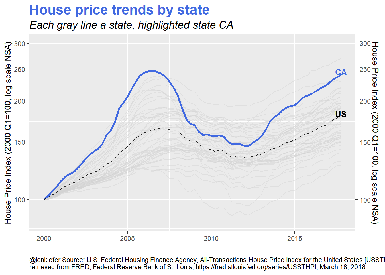
Here we show the US house price index and the California (CA) index. We also have the other states in faint gray lines.
What if we wanted to cycle through several states? Something like this?
Easy to do with tweenr. The following code will build this plot.
# tween states
# use keep_state to pause the animation for 10/15 frames

data <- dplyr::filter(df, state=="US") %>%
  keep_state(10) %>%
  tween_state(dplyr::filter(df, state=="CA"), 'linear', 10) %>%
  keep_state(15) %>%
  tween_state(dplyr::filter(df, state=="TX"), 'linear', 10) %>%
  keep_state(15) %>%
  tween_state(dplyr::filter(df, state=="FL"), 'linear', 10) %>%
  keep_state(15) %>%
  tween_state(dplyr::filter(df, state=="NY"), 'linear', 10) %>%
  keep_state(15) %>%
  tween_state(dplyr::filter(df, state=="OH"), 'linear', 10) %>%
  keep_state(15) %>%
  tween_state(filter(df, state=="US"), 'linear',10) %>%
  keep_state(10)

oopt = ani.options(interval = 1/10)
saveGIF({for (i in 1:max(data$.frame)) {
  df.plot<-dplyr::filter(data,.frame==i)
  p<-df.plot %>%
    ggplot(aes(x=date, y=hpi))+
    geom_line(data=df, aes(group=state),color="lightgray",alpha=0.5)+
    geom_line(size=1.1,color="royalblue") +
    geom_line(data=dplyr::filter(df,state=="US"),color="black",linetype=2, alpha=0.85)+
    geom_text(data=dplyr::filter(df,state=="US" & date==max(df.plot$date)), aes(label=state), nudge_y=0.01,fontface="bold",color="black",label="US")+
    geom_text(data=df.plot %>% filter(date==max(df.plot$date)), aes(label=state), nudge_y=0.01,fontface="bold",color="royalblue")+
    # set axis labels
    scale_y_log10(breaks=c(100,150,200,250,300),limits=c(85,300),sec.axis=dup_axis())+
    labs(x="",y="House Price Index (2000 Q1=100, log scale NSA)",
         title="House price trends by state",
         subtitle=paste("Each gray line a state, highlighted state",head(df.plot,1)$state),
         caption="@lenkiefer Source: U.S. Federal Housing Finance Agency, All-Transactions House Price Index for the United States [USSTHPI],\nretrieved from FRED, Federal Reserve Bank of St. Louis; https://fred.stlouisfed.org/series/USSTHPI, March 18, 2018.")+
    theme(plot.subtitle=element_text(face="italic",size=14),
          plot.title=element_text(color="royalblue",face="bold",size=18),
          plot.caption=element_text(hjust=0))
  print(p)

  print(paste0(i, " out of ",max(data$.frame)))

  ani.pause()}
},movie.name="YOURDIRECTORY/hpi1.gif",ani.width = 700, ani.height = 540) #replace YOURDIRECTORY with a place where you want to save the gif
There are two parts to this code. First, we take our data and use a combination of tween_state and keep_state to create the animation. The function tween_state interpolates between a beginning state (say the house price index for the U.S.) and an end state (say the house price index for CA). The function keep_state allows us to pause the animation.
The second part is a loop using the animation package’s saveGIF function along with some code to set up the plot.
Smooth time trend
We can also use tweenr to make a smooth animated line plot. Often for time series animations I won’t smooth them out, just letting the data reveal itselve frame-by-frame. And it works pretty well, see for example this simple example for reproducible code. But while updating my knowledge about tweenr, I ran across this nice example of animating a smooth linke plot using tweenr. Let’s apply that example to these data.
code for smooth plot
Here we’ll use a combination of tween_appear and tween_states to make the animation.
# modified from: https://www.kaggle.com/dmi3kno/leaderboard-shakeup-storyline-chart/code
df.us<-dplyr::filter(df,state=="US") %>%  select(date,hpi) %>%
  mutate(day=as.numeric(date-min(date)+1),ease="linear")

plot_data_tween<-tween_elements(df.us, time = "day",  group="ease", ease="ease", nframes = nrow(df.us)*5)
df_tween_appear <- tween_appear(plot_data_tween, time='day', nframes = nrow(df.us)*5)

# add pause at end of animation
df_tween_appear<- df_tween_appear %>% keep_state(20)

make_plot_appear <- function(i){
  plot_data <-
    df_tween_appear %>% filter(.frame==i, .age> -3.5)
  p<- plot_data %>%
    ggplot()+
    geom_line(aes(x=date, y=hpi),color="royalblue", size=1.3)+
    geom_point(data=. %>% filter(date==max(date)), mapping=aes(x=date, y=hpi), size=3,color="red",stroke=1.5)+
    geom_point(data=. %>% filter(date==max(date)), mapping=aes(x=date, y=hpi), color="white", size=2)+
    geom_text(data=. %>% filter(date==max(date)), mapping=aes(x=date, y=hpi,label=round(hpi,0)),color="red",nudge_x=7,hjust=-0.4,fontface="bold")+
    geom_line(data=df.us, aes(x=date,y=hpi),alpha=0.1)+
    theme_minimal(base_family = "sans")+
    scale_x_date(limits = c(as.Date("2000-01-01"),as.Date("2018-04-30")),
                     date_breaks = "1 year",date_labels="%Y")  +
    scale_y_continuous(sec.axis=dup_axis())+
    theme(plot.subtitle=element_text(face="italic",size=14),
          plot.title=element_text(color="royalblue",face="bold",size=18),
          plot.caption=element_text(hjust=0),
          panel.grid.major.x = element_line(color="lightgray"),
          panel.grid.minor.x = element_line(color="lightgray"),
          panel.grid.major.y = element_line(color="lightgray"),
          panel.grid.minor.y = element_line(color="lightgray"))+
    labs(x="",y="House Price Index (2000 Q1=100, log scale NSA)",
         title="U.S. house price index",
         subtitle="(2000 Q1 =1 100)",
                 caption="@lenkiefer Source: U.S. Federal Housing Finance Agency, All-Transactions House Price Index for the United States [USSTHPI],\nretrieved from FRED, Federal Reserve Bank of St. Louis; https://fred.stlouisfed.org/series/USSTHPI, March 18, 2018.")
  return(p)
}

oopt<-ani.options(interval=1/20)
saveGIF({for (i in 1:max(df_tween_appear$.frame)){
  g<-make_plot_appear(i)
  print(g)
  print(paste(i,"out of",max(df_tween_appear$.frame)))
  ani.pause()
}
},movie.name="YOURDIRECTORY/hpi2.gif",ani.width = 700, ani.height = 540)
Resulting in:
We also might want to compare several states, so we can easily modify our code like so:
# now compare US, CA and TX
df.us2<-dplyr::filter(df,state %in% c("TX","CA","US")) %>%  select(date,state,hpi) %>%
  mutate(day=as.numeric(date-min(date)+1),ease="linear")


plot_data_tween2<-tween_elements(df.us2, time = "day",  group="state", ease="ease", nframes = nrow(df.us2))
df_tween_appear2 <- tween_appear(plot_data_tween2, time='day', nframes = nrow(df.us2))
#df_tween_appear$date <- as.POSIXct(as.Date("2000-01-01")+df_tween_appear$day)

# add pause at end of animation
df_tween_appear2<- df_tween_appear2 %>% keep_state(20)
summary(df_tween_appear2)
#filter(df_tween_appear, .frame==334 & date>"2018-03-01")

make_plot_appear2 <- function(i){
  plot_data <-
    df_tween_appear2 %>% filter(.frame==i, .age> -3.5)
  p<- plot_data %>%
    ggplot()+
    geom_line(aes(x=date, y=hpi, color=.group), size=1.3)+
    geom_point(data=. %>% filter(date==max(date)), mapping=aes(x=date, y=hpi,color=.group), size=3,stroke=1.5)+
    geom_point(data=. %>% filter(date==max(date)), mapping=aes(x=date, y=hpi,color=.group),  size=2)+
    geom_text(data=. %>% filter(date==max(date)), mapping=aes(x=date, y=hpi,label=.group, color=.group),nudge_x=7,hjust=-0.4,fontface="bold")+
    geom_line(data=df.us2, aes(x=date,y=hpi, group=state),alpha=0.25,color="darkgray")+
    theme_minimal(base_family = "sans")+
    scale_x_date(limits = c(as.Date("2000-01-01"),as.Date("2018-04-30")),
                 date_breaks = "1 year",date_labels="%Y")  +
    scale_y_continuous(sec.axis=dup_axis())+
    theme(plot.subtitle=element_text(face="italic",size=14),
          legend.position="none",
          plot.title=element_text(color="royalblue",face="bold",size=18),
          plot.caption=element_text(hjust=0),
          panel.grid.major.x = element_line(color="lightgray"),
          panel.grid.minor.x = element_line(color="lightgray"),
          panel.grid.major.y = element_line(color="lightgray"),
          panel.grid.minor.y = element_line(color="lightgray"))+
    labs(x="",y="House Price Index (2000 Q1=100, log scale NSA)",
         title="House price index",
         subtitle="(2000 Q1 =1 100)",
         caption="@lenkiefer Source: U.S. Federal Housing Finance Agency, All-Transactions House Price Index ,\nretrieved from FRED, Federal Reserve Bank of St. Louis; https://fred.stlouisfed.org/series/XXSTHPI, March 18, 2018. [XX= state code or US]")
  return(p)
}

oopt<-ani.options(interval=1/20)
saveGIF({for (i in 1:max(df_tween_appear2$.frame)){
  g<-make_plot_appear2(i)
  print(g)
  print(paste(i,"out of",max(df_tween_appear2$.frame)))
  ani.pause()
}
},movie.name="YOURDIRECTORY/hpi3.gif",ani.width = 700, ani.height = 540)
to produce this plot.
Carnival Horse Race Plot
Finally, we can recreate my horse race animated dotplot. This plot compares the level of the house price index by state over time.
df.state2 <-df %>% mutate(state=as.factor(state), date=as.factor(date)) %>%   select(date,state,hpi) %>% group_by(state) %>%
  mutate(hpilag12=c(lag(hpi,4))) %>% ungroup()

myf<-function(y=2012) {
  filter(df.state2,year(date)==y & month(date)==10) %>% data.frame()
}

mylist<-lapply(c(2000:2017,2000),myf)
tween.df<-tween_states(mylist,tweenlength=3,statelength=2, ease=rep('cubic-in-out',11), nframes=250)


plotf3<- function(i=1){
  g<-
    tween.df %>% filter(.frame==i) %>%
    ggplot(aes(x=hpi, y=state, label=state))+
    geom_text(nudge_x = 0.025,color="royalblue")  +
    geom_point(color="royalblue",size=3)+
    scale_x_log10(limits=c(70,300), breaks=c(70,100,150,200,250,300))+
    geom_segment(aes(xend=hpilag12,x=hpi,y=state,yend=state),alpha=0.7)+
    theme_minimal()  +
    labs(y="State", x="House price index (log scale, 2000 Q1 =100, NSA)",
         title="State house price dynamics",
         subtitle=paste0("Q4 of ",as.character(as.Date( tail(tween.df  %>% filter(.frame==i),1)$date), format="%Y")," line 4-quarter lag\n"),
         caption="@lenkiefer Source: U.S. Federal Housing Finance Agency, All-Transactions House Price Index,\nretrieved from FRED, Federal Reserve Bank of St. Louis;\nhttps://fred.stlouisfed.org/series/XXSTHPI, March 18, 2018. [XX= state code or US]")+
    theme(plot.title=element_text(size=18,color="royalblue",face="bold"),
          plot.subtitle=element_text(size=14,face="italic"),
          plot.caption=element_text(hjust=0,vjust=1),
          axis.text.x=element_text(size=12),
          legend.key.width=unit(1,"cm"),
          legend.position="top",
          axis.text.y=element_blank(),
          axis.title.y=element_blank(),
          panel.grid.major.y =element_blank())
}

saveGIF({for (i in 1:max(tween.df$.frame)){
  #  saveGIF({for (i in 1:20){
  g<-plotf3(i)
  print(g)
  print(paste(i,"out of",max(tween.df$.frame)))
  ani.pause()
}
},movie.name="YOURDIRECTORY/hpi4.gif", ani.width=650, ani.height=800)
More to do
There’s stil more to do. The new tween_state function has enter and exit arguments that supposedly allow for d3.js-like entry and exit effects. But I haven’t been able to figure out exactly how to use them. When I do, perhaps it will be time for a follow-up post.