LET’S PICK BACK UP where we left off and think about communicating forecast results. To help guide our thinking, let’s set up a little game.
Basic setup
Like last time we’re going to focus on a situation where a forecaster observes some information about the world and makes an announcement about a future binary outcome. A decision maker observes the forecaster’s announcement and takes a binary action. Then the outcome is realized and the forecaster receives a payoff. The decision maker’s action will be a mechanical function of the forecaster’s announcement.
We have:
- Y: an outcome, either 0 or 1
- X: an observation about the world. For simplicity we’ll assume that the forecaster observes P(Y|X) which corresponds to an unbiased estimate of the conditional probability of the outcome taking place
- A: an action, either 0 or 1
- Z: a signal from the forecaster, a value between 0 and 1 (e.g. a pronouncement of the forecaster’s assessment of the conditional likelihood that Y=1)
Forecaster payoffs
We’ll need to parameterize the forecaster’s payoffs. I’ve chosen a particular functional form which has the following properties.
- The forecaster’s payoff depends on the pronouncement Z, the action taken A, and the outcome Y
- The closer the pronouncement is to the true outcome, the lesser the payoff. The payoff takes a quadratic form.
- The right action (A= 0 when Y =0 or A =1 to Y =1) is always better
- The payoff is symmetric
Having the payoff depend on the pronouncement rather than solely the outcomes captures a reputation effect. All else being equal, the forecaster would prefer to be right.
Let’s simulate this payoff and take a look. Per usual, we’ll generate the figures and analysis with R.
The code below generates the following three graphs which help illustrate the payoffs.
#####################################################################################
## Step 0: Load libraries ###
#####################################################################################
library(tidyverse)
library(ggridges)
library(viridis)

#####################################################################################
## Step 2: set parameters ###
#####################################################################################
X    <- seq(0,1,.1)    # probabilities
Z    <- seq(0,1,.1)    # signals
a    <- c(0,1)         # actions
y    <- c(0,1)         # outcomes
c1   <- 0.5            # payoff parameter 1
c2   <- 0.5            # payoff parameter 2
ccd  <- 0.5            # cutoff on decision
mx11 <- 0.3            # relative rate on reputation (getting it right)
mx22 <- 0.3            # relative rate on repurtation (getting it right)
mx12 <- 0.1            # relative rate on reputation (getting it right)
mx21 <- 0.1            # relative rate on reputation (getting it right)


#####################################################################################
## Step 3: analyze ###
#####################################################################################

# Simulate some information, signals, actions, and outcomes
df2<-expand.grid(x=X,z=Z, a=a,y=y)

# Function to compute forecaster payoffs

f.payoff3<- function(y=0,a=0,z=0,cc1=c1,cc2=c2,m11=mx11,m22=mx22,m12=mx12,m21=mx21,...){
  payoff<-case_when(y==0 & a==0 ~ -m11*(z>0.5)*(z-0.5)**2-m21*abs(z-y),
                    y==0 & a==1 ~ -cc2-sign(z-0.5)*(z-0.5)**2,
                    y==1 & a==1 ~ -m22*(z<0.5)*(0.5-z)**2-m12*abs(z-y),
                    y==1 & a==0 ~ -cc1-sign(0.5-z)*(z-0.5)**2
  )
  return(payoff)
}

# Simulate payoffs using purrr::pmap

df2 %>%  as.tbl() %>% mutate(payoff= pmap(list(y=y,a=a,z=z),f.payoff3, cc1=c1,cc2=c2)) %>% unnest() %>%
  mutate(outcome=paste0("Action A = ",a,", outcome Y = ",y))-> df4

# plot payoffs

ggplot(data=df4, aes(x=z,y=payoff, color=outcome))+geom_line(size=1.1)+theme_gray()+
  scale_color_viridis(option="D",discrete=T,end=0.85)+
  labs(x="Signal ",y="Forecaster Payoff",
       title="Payoffs given signal Z, action A, and outcome Y",
       subtitle="Action A = 1 taken if Z >= c, A=0 if Z < c")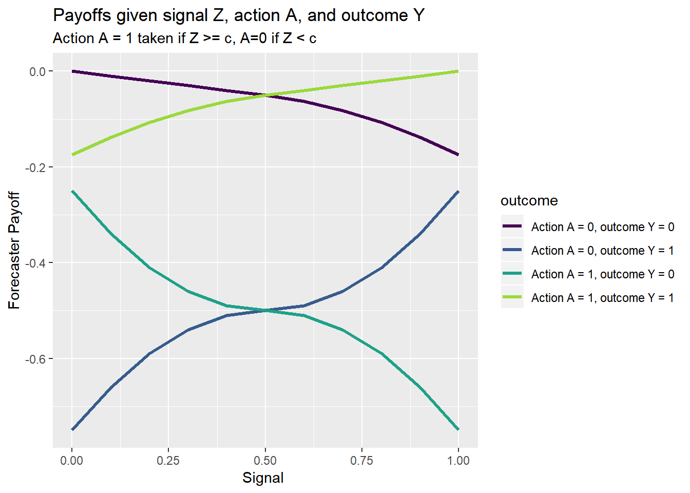
ggplot(data=df4, aes(x=z,y=payoff, color=outcome,group=outcome))+
  theme_gray()+facet_wrap(~outcome,scales="free_x")+scale_y_continuous(sec.axis=dup_axis())+
  geom_line(data=df4 %>% mutate(outcome=NULL), aes(group=paste(a,y)),size=1.1,color="gray",alpha=0.85)+
  geom_line(size=1.1)+
  scale_color_viridis(option="D",discrete=T,end=0.85)+
  labs(x="Signal ",y="Forecaster Payoff",
       title="Payoffs given signal Z, action A, and outcome Y",
       subtitle="Action A = 1 taken if Z >= c, A=0 if Z < c")+
  theme(legend.position="none")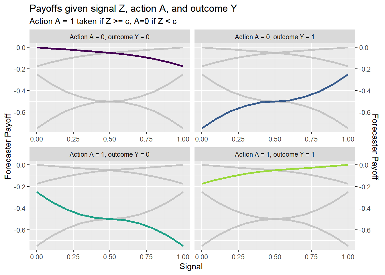
ggplot(data=df4, aes(x=z,y=payoff, color=outcome,group=outcome))+
geom_line(alpha=0)+
geom_line(size=1.1,color="gray",alpha=0.85)+
theme_gray()+
geom_line(data=filter(df4, a==1 & y==0),size=1.1)+
geom_text(data=filter(df4, a==1 & y==0 & z==0.5), aes(label=outcome,y=-0.4))+
scale_color_viridis(option="D",discrete=T,end=0.85)+
labs(x="Signal ",y="Forecaster Payoff",
title="Payoffs given signal Z, action A, and outcome Y",
subtitle="Action A = 1 taken if Z >= c, A=0 if Z < c")+
theme(legend.position="none")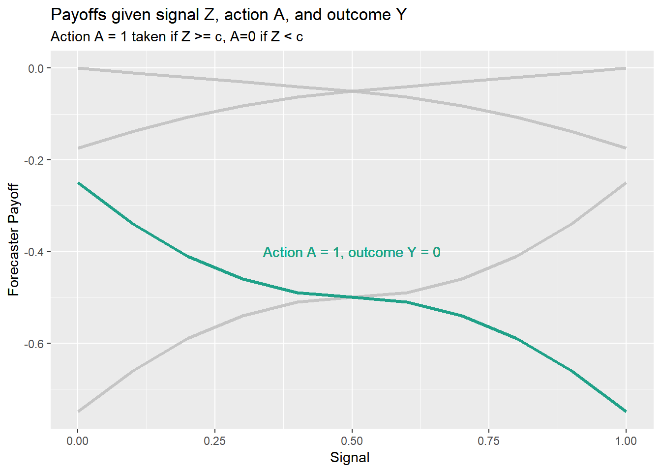 Given this payoff structure, what’s the best thing for the forecaster to do? Well, it depends on how actions are decided. For now, let’s assume that the action A depends solely on the forecaster’s signal Z. If Z is greater or equal to some cutoff c, then the action A=1 is taken, otherwise action A=0 is taken. The following code allows us to determine the optimal response Z, conditional on information X and cutoff c.
We can also plot the optimal Z as a function of these variables. Below I try several representations.
# Function for expected payoffs

f.payoff5<- function(zz=0,  # signal
                     xx=0,  # information
                     ccd=cd # cutoff
                     ,...){
  payoff5<- xx*f.payoff3(y=1,a=1*(zz>=ccd),z=zz) + (1-xx)*f.payoff3(y=0,a=1*(zz>=ccd),z=zz)
  return(payoff5)
}


# optimize over signal z:
optz<- function(xt=0, ct=cd){
  return(optimize(f.payoff5,c(0,1),xx=xt,ccd=ct,maximum=TRUE,tol=.Machine$double.eps^0.25)$maximum)
}


#data.frame(expand.grid(y=c(0,1), z=c(0,1))) %>% mutate(payoff=pmap(list(y=y,z=z,a=1*(z==1)), f.payoff3)) %>% unnest() -> df6

data.frame(expand.grid(x=seq(0,1,.02),cd=seq(0,1,.1))) %>% mutate(zstar=map2(x,cd,optz)) %>% unnest()->dfz

# plot results

ggplot(data=dfz, aes(x=x,y=cd,fill=zstar))+geom_tile(color=NA)+scale_fill_viridis(option="B",name="Signal Z")+
  labs(x="Observed P(Y=1|X)",y="Cutoff c, defining action A: A=I(Z >= c)", title="Optimal Signal Z, conditional on P(Y=1|X) and cutoff c",
       subtitle="Action A = 1 taken if Z >= c, A=0 if Z < c")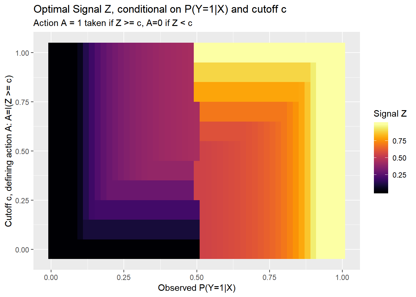
ggplot(data=dfz, aes(x=x,y=zstar))+geom_line() + geom_line(linetype=2,color="darkgray",aes(y=x))+facet_wrap(~cd) +
  labs(x="Observed P(Y=1|X)",y="Signal Z", title="Optimal Signal Z, conditional on P(Y=1|X) and cutoff c",
       subtitle="Action A = 1 taken if Z >= c, A=0 if Z < c")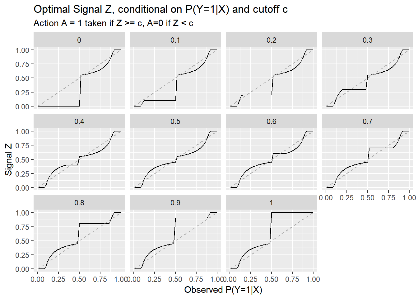
ggplot(data=dfz, aes(x=x,height=zstar,y=0,fill=zstar))+
  geom_ridgeline_gradient(color="black")+facet_wrap(~paste("c =",cd))+scale_fill_viridis(option="B",name="Response Z")+
  geom_line(aes(y=x),color="darkgray",linetype=2) +
  labs(x="Observed P(Y=1|X)",y="Signal Z", title="Optimal Signal Z, conditional on P(Y=1|X) and cutoff c",
       subtitle="Action A = 1 taken if Z >= c, A=0 if Z < c")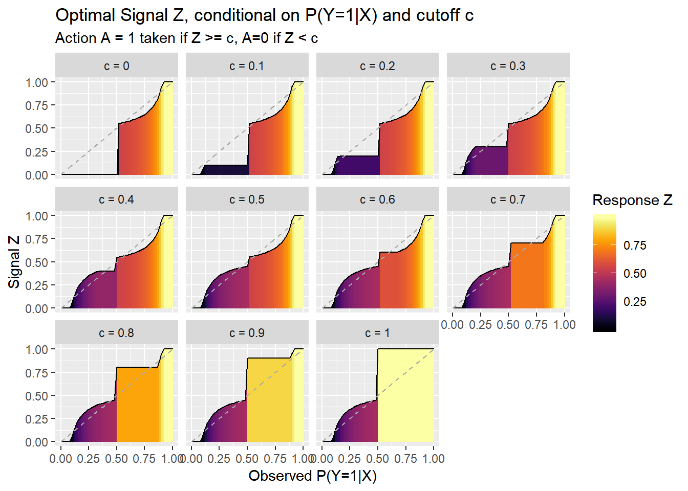
ggplot(data=dfz, aes(x=x,height=zstar-x,y=x,fill=zstar-x))+
  geom_ridgeline_gradient(color="black",min_height=-1)+
  facet_wrap(~paste("c =",cd))+
  scale_fill_viridis(option="B",name="Response Z")+
  geom_line(aes(y=x),color="darkgray",linetype=2) +
  labs(x="Observed P(Y=1|X)",y="Signal Z", title="Optimal Signal Z, conditional on P(Y=1|X) and cutoff c",
       subtitle="Action A = 1 taken if Z >= c, A=0 if Z < c")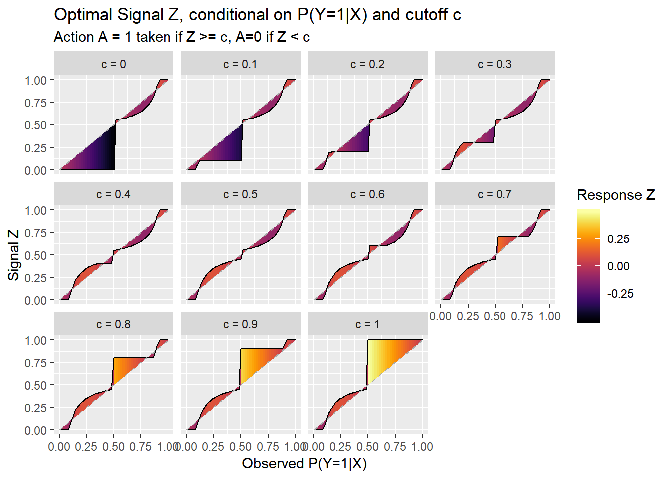
Discussion
These charts show that the optimal signal is not always equal to the best estimate of the conditional probability. The best response is no longer a step function see our earlier results. Now, due to reputation effects, the forecaster seeks to hedge, particularly in cases where a specific action is going to be taken regardless of what the forecaster says (c=0 or c=1).
It’s also interesting to look at the case when c=0.5.
Expected payoffs
In this setup, how does the forecaster’s expected payoff vary as a function of information X?
Let’s plot it:
# compute expected payoffs

dfz %>% mutate(ep=pmap(list(zz=zstar,xx=x,ccd=cd),f.payoff5)) %>% unnest() -> dfz2


ggplot(data=dfz2, aes(x=x,height=zstar,y=0,fill=ep))+
  geom_ridgeline_gradient(color="black")+facet_wrap(~paste("c =",cd))+scale_fill_viridis(option="B",name="Response Z")+
  geom_line(aes(y=x),color="darkgray",linetype=2) +
  labs(x="Observed P(Y=1|X)",y="Expected Payoff", title="Expected Payoff given optimal Signal Z, conditional on P(Y=1|X) and cutoff c",
       subtitle="Action A = 1 taken if Z >= c, A=0 if Z < c")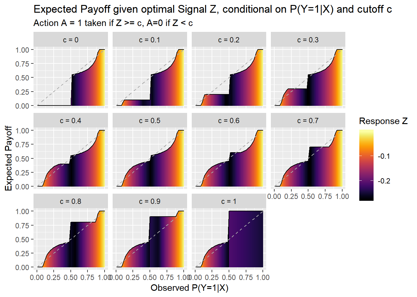
ggplot(data=dfz2, aes(x=x,height=zstar-x,y=x,fill=ep))+
  geom_ridgeline_gradient(color="black",min_height=-1)+facet_wrap(~paste("c =",cd))+scale_fill_viridis(option="B",name="Response Z")+
  geom_line(aes(y=x),color="darkgray",linetype=2) +
  labs(x="Observed P(Y=1|X)",y="Expected Payoff", title="Expected Payoff given optimal Signal Z, conditional on P(Y=1|X) and cutoff c",
       subtitle="Action A = 1 taken if Z >= c, A=0 if Z < c")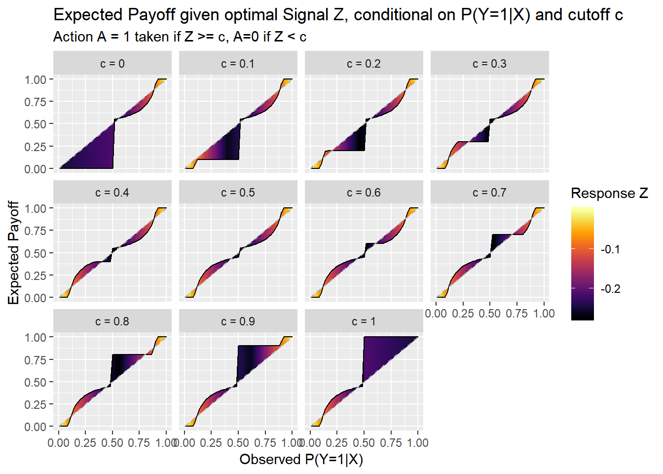
ggplot(data=dfz2, aes(x=x,y=cd,fill=ep))+geom_tile(color=NA)+scale_fill_viridis(option="B",name="Signal Z")+
  labs(x="Observed P(Y=1|X)",y="Cutoff c, defining action A: A=I(Z >= c)", title="Expected payoff given optimal Signal Z, conditional on P(Y=1|X) and cutoff c",
       subtitle="Action A = 1 taken if Z >= c, A=0 if Z < c")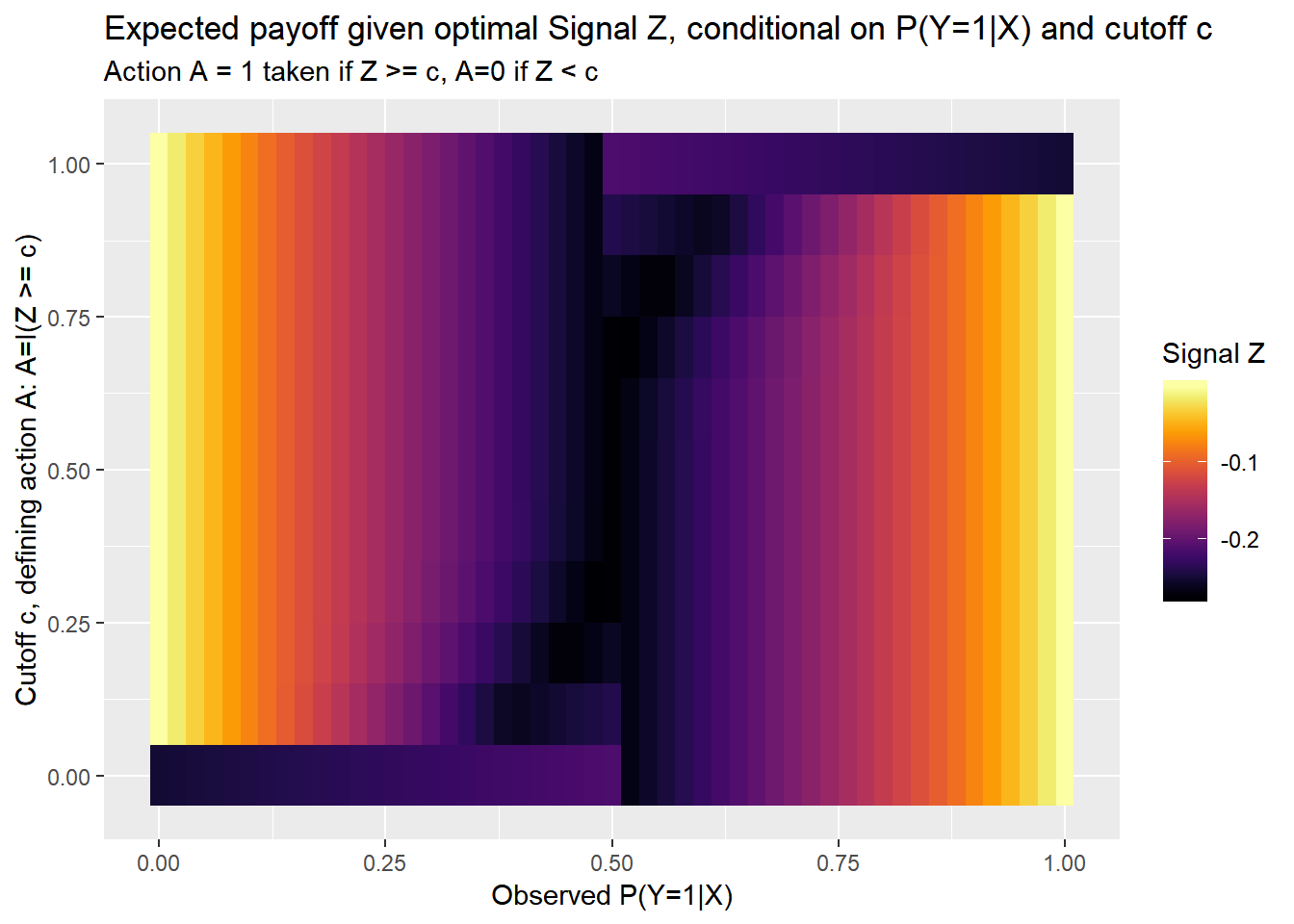
Here we can see that the payoff is generally greater when there is less uncertainty around Y. Very high, or very low conditional probabilities allow the forecaster to make a strong pronouncement with greater confidence.
Next steps
We still haven’t answered how the decision maker might respond given the forecaster’s behavior. But we can expand this example to figure out the best cutoff for the decision maker to set.