The Vector Error Correction Model

The VECM is a useful tool for forecasting variables with a stochastic trend. This sort of thing comes up all the time in macroeconomics. Lütkepohl, H. (2005) or Hamilton (1994) provide textbook treatments. For this case, we’ll consider a bivariate system of two variables. We can write it as:

\[ \begin{bmatrix} \Delta y_t \\ \Delta x_t \end{bmatrix} = \alpha \beta' \begin{bmatrix} y_{t-1} \\ x_{t-1} \end{bmatrix} + \sum_i^p \Gamma_i \begin{bmatrix} \Delta y_{t-i} \\ \Delta x_{t-i} \end{bmatrix} +\epsilon_t \] Where \(\beta\) is the cointegrating vector.

There is a large literature on estimating these models. See references at the end for an introduction.

Forecasting

One use of such models is to forecast. If we were in a standard case, where we had the same number of observations for \(y\) and \(x\) we could translate the VECM into a Vector AutoRegression (VAR) and forecast from the VAR. The vars and urca packages can handle this case.

But what if we had observations on \(x\) (or perhaps forecasts we really really believed)? How can we construct forecasts for \(y\) conditional on these forecasts? That’s what we’re going to do here.

A simulation

Here’s the code for a little simulation.

The idea is to estimate a VECM with tsDyn::VECM, and then to cast it into VAR form using tsDyn::VARrep. Then you set up a state space model using KFAS and then feed the observations into the state space model. For periods where \(x\) is observed by \(y\) is not, you feed the state space model missing values.

# Bivariate VECM conditional forecasts
set.seed(1031)

library(forecast)
library(KFAS)
library(tidyverse)
library(vars)
library(cointReg)
library(tsDyn)


### SIMULATE DATA 

# in-sample size
N1 <- 40 

# hold-out sample
N2 <- 20
N <- N1+N2

# Cointegration vector is (1, -betaX)
betaX=2  
sigu =1
sige =1

# Simulate process
# simulation process similar to one in

# Vogelsang, T. J., & Wagner, M. (2014). Integrated modified OLS estimation and fixed-b inference for cointegrating regressions. Journal of Econometrics, 178(2), 741-760.

# y_t = my_y+ betaX*x_t + eps_t
# x_t = mu_x+ x_(t-1) + nu_t
# nu_t = e_t + rhox * e_(t-1)
# eps_t = rhoy *eps_(t-1) + u_t + gamma1 * e_t

# u_t ~ N(0,sigu**2)
# e_t ~ N(0,sige**2)

et <- rnorm(N,0,sige)
ut <- rnorm(N,0,sigu)

rhox <- 0.5
rhoy <- 0.3

mu_y <- 0.1
mu_x <- 0.01

#degree of endogeneity indexed by gamma
gamma1 <- 0.3 

# simulate X, Y

y <- rep(0,N)
x <- rep(0,N)

x[1]  <- et[1]
nu    <- rep(0,N)
nu[1] <- et[1]

epst <- rep(0,N)
epst[1] <- ut[1] + gamma1*et[1]

for (i in 2:N){
  nu[i] <- et[i] + rhox* et[i-1]
  x[i] <- mu_x + x[i-1] + nu[i]
  epst[i] <- rhoy*epst[i]+ut[i] + gamma1* et[i]
  y[i] <- mu_y + betaX* x[i]+epst[i]
}

# all observations
yx <- ts.union(ts(y),ts(x))
# in sample time series
yx1 <- window(yx, end=N1)
# out of sample period
yx2 <- window(yx,start=N1+1)

plot our simulated series

autoplot(yx2) + labs(title="Simulated cointegrated series {y,x} ")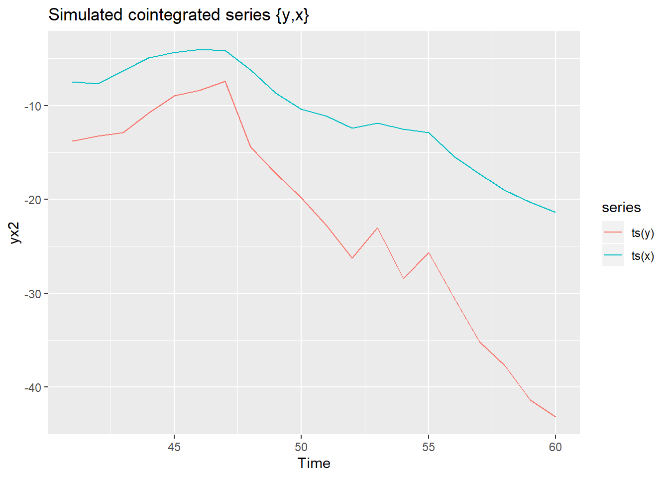

Figure 1: Simulated Cointegrated Series

With our simulated data we can estimate a VECM and convert to VAR representation:

# estimate vecm1
vecm1 <- VECM(yx1,lag=1)

vecm1 %>% summary()

## #############
## ###Model VECM 
## #############
## Full sample size: 40     End sample size: 38
## Number of variables: 2   Number of estimated slope parameters 8
## AIC 5.170909     BIC 19.90918    SSR 240.6511
## Cointegrating vector (estimated by 2OLS):
##    ts(y)     ts(x)
## r1     1 -2.060931
## 
## 
##                ECT                 Intercept           ts(y) -1           
## Equation ts(y) -0.5429(0.6096)     -0.3511(0.4096)     -0.6044(0.4144)    
## Equation ts(x) 0.1202(0.2466)      -0.1099(0.1657)     -0.2070(0.1676)    
##                ts(x) -1         
## Equation ts(y) 2.4040(0.9317)*  
## Equation ts(x) 1.0065(0.3768)*

# VAR reprecsentation of VECM
VARrep(vecm1)

##         constant    ts(y).l1 ts(x).l1  ts(y).l2  ts(x).l2
## ts(y) -0.3510998 -0.14721608 3.522812 0.6043504 -2.404003
## ts(x) -0.1098973 -0.08677976 1.758797 0.2069827 -1.006527

Now that we have a VAR representation, we can convert it to a state space representation. We will follow the KFAS notation and set up the following equations:

\[ y_t = Z_t \alpha_t + \epsilon_t \]

\[ \alpha_t = T_t \alpha_{t-1} + R_t \eta_t \] with \(\epsilon_t \sim N(0,H_t)\) and \(\eta_t \sim N(0,Q_t)\).

We can get \(T_t\) and \(Q_t\) from the VAR plus and specify \(Z_t\) based on the structure of our setup.

# initialize yx_miss to hold our data
yx_miss <- yx

#y is missing from period N1+1 forward, replace with NA

yx_miss[(N1+1):N,1] <- NA

# plot simulated data
autoplot(yx_miss) + labs(title="Cointegrated series {y,x} with y missing after period N1 (=40)")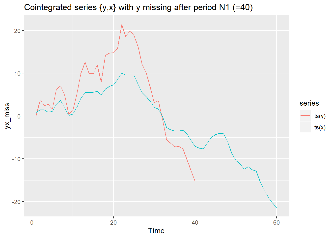

Figure 2: Cointegrated series {y,x}, with missing observations for y

In this setup we observe y until period 40, but continue to observe x until the end of our sample at period 60. We might have literally observed x, or we might have a very reliable forecast and we want to condition our estimate of y on that forecast. A statespace model can help us do it.

# Set up statespace model
#extract intercept from VAR

intercept <- VARrep(vecm1)[,1]

# observation is just x,y
Ft <- cbind(diag(1,2),diag(0,2))

#transiton equation for VAR, based on estimate VECM coefficients (after converted to VAR)
Tt <-
  matrix(c(VARrep(vecm1)[1,-1],
           VARrep(vecm1)[2,-1],
           c(1,0,0,0),
           c(0,1,0,0)),
         nrow=4,byrow=TRUE)

# residuals variance matrix from VECM

Qt <- cov(residuals(vecm1))


# set up statespace model

K2 <- SSModel( yx_miss~ -1 +
                 # add the intercept 
                SSMcustom(Z = diag(0,2), T = diag(2), Q = diag(0,2), 
                          a1 = matrix(intercept,2,1), P1inf = diag(0,2),index=c(1,2),
                          state_names=c("mu_y","mu_x"))+
                 
                 # add the VAR part (excluding intercept)
                 
                 SSMcustom(Z=Ft,  # observations
                           
                           T=Tt, # state transtion (from VECM)
                           
                           Q=Qt,  # state innovation variance (from VECM)
                           
                           index=c(1,2), # we observe variables 1 & 2 from statespace (without noise)
                           
                           
                           state_names=c("y","x","ylag","xlag"),  # name variables
                           
                           a1=c(y[2],x[2],y[1],x[1]),   #initialize values
                           
                           P1=1e7*diag(1,4)),  # make initial variance very large
               
               H=diag(0,2) # no noise in observation equation
               )


# Predict values for our statespace model
predict(K2,interval = "confidence", level = 0.95 )[[1]] %>% 
  #convert to time series
  ts %>% 
  # plot
  autoplot()+autolayer(yx[,1],color="black")+
  scale_color_manual(values=c("red","blue","blue"))+
  labs(x="periods",y="y",
       title="Forecasts for y conditional on x",
       subtitle="y and x are bivariate VECM, x observed after period 40, y is not")+
  geom_vline(xintercept=40,linetype=2)+
  annotate(geom="text",x=40.5,y=0, label="Forecasts for X available, \nY unobserved",hjust=0)

## Warning in sqrt(out$V_mu[i, i, timespan]): NaNs produced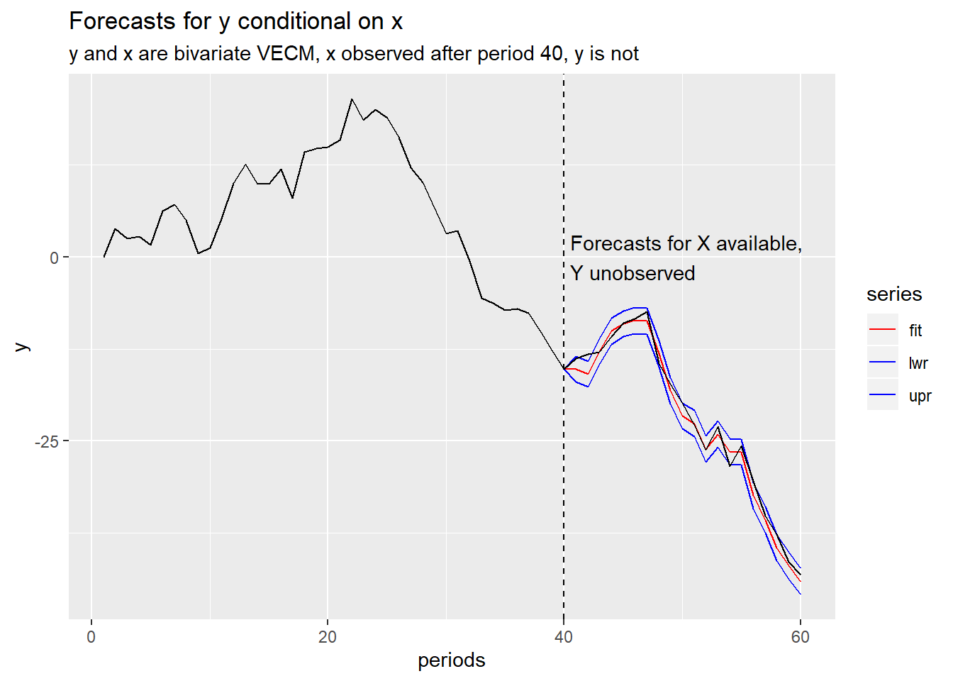

Figure 3: VECM Forecasts from Statespace Model

In the plot above the red line is the conditional forecast while the blue lines are the upper and lower bounds.

This seems like it’s working.

What can we do with this? Well, that’s something we will explore next time.

References

Hamilton, J. D. (1994). Time series analysis. Princeton University Press, USA.

Lütkepohl, H. (2005). New introduction to multiple time series analysis. Springer Science & Business Media.