Recently the U.S. Census Bureau released updated population estimates through 2018 for the United States, states, counties, and metropolitan statistical areas (MSA). Press release
I tweeted out the following chart comparing house prices and state population dynamics.
demographics are an important driver of #housing market trends.
— 📈 Len Kiefer 📊 (@lenkiefer) May 1, 2019
here's a comparison of growth in state population and nominal house prices
since the year 2000
left to right: more people
bottom to top: higher home prices pic.twitter.com/CtliCFrWoG
In this post, I was to dig a little deeper, comparing various aspects of population dynamics to house price trends. We’ll analyze things a the MSA level. Per usual we will use R and include code tucked away between the arrows like so:
Click for code
Hello!
Data
Get Data
The latest population estimates from 2010 to 2018 for metro areas can be found here. We’ll download the .csv file with the data directly into R. We’ll also get house prices using the Freddie Mac House Price Index. We can also read in the house price data as a .csv. We’ll use the data.table package fread function to get the data into R.
Data Download Code
# libraries ----
library(tidyverse)
library(data.table)
library(ggrepel)
library(scales)
# get data ----
df <- fread("https://www2.census.gov/programs-surveys/popest/datasets/2010-2018/metro/totals/cbsa-est2018-alldata.csv")
df_hpi <- fread("http://www.freddiemac.com/fmac-resources/research/docs/fmhpi_master_file.csv")
Wrangle Data
Now that we have our data, we need to do a bit of wrangling. Details hidden below.
Data Wrangling Code
Population data
Let’s take a look at our population data as it comes from Census. Details of the file layout are available in this pdf file.
str(df)## Classes 'data.table' and 'data.frame': 2789 obs. of 88 variables:
## $ CBSA : int 10180 10180 10180 10180 10420 10420 10420 10500 10500 10500 ...
## $ MDIV : int NA NA NA NA NA NA NA NA NA NA ...
## $ STCOU : int NA 48059 48253 48441 NA 39133 39153 NA 13007 13095 ...
## $ NAME : chr "Abilene, TX" "Callahan County, TX" "Jones County, TX" "Taylor County, TX" ...
## $ LSAD : chr "Metropolitan Statistical Area" "County or equivalent" "County or equivalent" "County or equivalent" ...
## $ CENSUS2010POP : int 165252 13544 20202 131506 703200 161419 541781 157308 3451 94565 ...
## $ ESTIMATESBASE2010 : int 165246 13546 20192 131508 703203 161425 541778 157493 3451 94562 ...
## $ POPESTIMATE2010 : int 165583 13513 20237 131833 703035 161389 541646 157589 3435 94513 ...
## $ POPESTIMATE2011 : int 166616 13511 20266 132839 703123 161857 541266 157853 3315 95046 ...
## $ POPESTIMATE2012 : int 167447 13488 19870 134089 702080 161375 540705 157349 3376 94676 ...
## $ POPESTIMATE2013 : int 167472 13501 20034 133937 703625 161691 541934 156019 3351 93391 ...
## $ POPESTIMATE2014 : int 168355 13506 19846 135003 704921 162459 542462 155248 3292 92720 ...
## $ POPESTIMATE2015 : int 169704 13591 19972 136141 704448 162615 541833 153604 3196 91495 ...
## $ POPESTIMATE2016 : int 170018 13789 19969 136260 703690 162595 541095 152353 3186 90371 ...
## $ POPESTIMATE2017 : int 170516 13968 19852 136696 704367 162625 541742 151293 3180 89417 ...
## $ POPESTIMATE2018 : int 171451 13994 19817 137640 704845 162927 541918 153009 3092 91243 ...
## $ NPOPCHG2010 : int 337 -33 45 325 -168 -36 -132 96 -16 -49 ...
## $ NPOPCHG2011 : int 1033 -2 29 1006 88 468 -380 264 -120 533 ...
## $ NPOPCHG2012 : int 831 -23 -396 1250 -1043 -482 -561 -504 61 -370 ...
## $ NPOPCHG2013 : int 25 13 164 -152 1545 316 1229 -1330 -25 -1285 ...
## $ NPOPCHG2014 : int 883 5 -188 1066 1296 768 528 -771 -59 -671 ...
## $ NPOPCHG2015 : int 1349 85 126 1138 -473 156 -629 -1644 -96 -1225 ...
## $ NPOPCHG2016 : int 314 198 -3 119 -758 -20 -738 -1251 -10 -1124 ...
## $ NPOPCHG2017 : int 498 179 -117 436 677 30 647 -1060 -6 -954 ...
## $ NPOPCHG2018 : int 935 26 -35 944 478 302 176 1716 -88 1826 ...
## $ BIRTHS2010 : int 540 31 25 484 1977 407 1570 545 4 381 ...
## $ BIRTHS2011 : int 2295 120 154 2021 7568 1500 6068 2334 35 1569 ...
## $ BIRTHS2012 : int 2358 122 189 2047 7497 1381 6116 2183 37 1385 ...
## $ BIRTHS2013 : int 2390 135 189 2066 7545 1420 6125 2211 31 1403 ...
## $ BIRTHS2014 : int 2382 140 180 2062 7704 1504 6200 2061 25 1275 ...
## $ BIRTHS2015 : int 2417 153 159 2105 7562 1476 6086 2032 38 1279 ...
## $ BIRTHS2016 : int 2379 152 157 2070 7450 1417 6033 1938 28 1223 ...
## $ BIRTHS2017 : int 2427 163 170 2094 7308 1374 5934 1900 33 1205 ...
## $ BIRTHS2018 : int 2381 159 164 2058 7212 1370 5842 1844 30 1203 ...
## $ DEATHS2010 : int 406 60 21 325 1605 336 1269 410 2 267 ...
## $ DEATHS2011 : int 1506 158 213 1135 6662 1292 5370 1242 27 761 ...
## $ DEATHS2012 : int 1587 142 173 1272 7011 1365 5646 1396 16 894 ...
## $ DEATHS2013 : int 1694 176 206 1312 6991 1378 5613 1461 25 924 ...
## $ DEATHS2014 : int 1598 178 196 1224 6851 1372 5479 1414 23 851 ...
## $ DEATHS2015 : int 1698 168 202 1328 7453 1457 5996 1452 44 876 ...
## $ DEATHS2016 : int 1726 192 189 1345 7286 1474 5812 1528 31 974 ...
## $ DEATHS2017 : int 1705 174 188 1343 7283 1444 5839 1528 27 950 ...
## $ DEATHS2018 : int 1739 183 172 1384 7229 1434 5795 1561 27 950 ...
## $ NATURALINC2010 : int 134 -29 4 159 372 71 301 135 2 114 ...
## $ NATURALINC2011 : int 789 -38 -59 886 906 208 698 1092 8 808 ...
## $ NATURALINC2012 : int 771 -20 16 775 486 16 470 787 21 491 ...
## $ NATURALINC2013 : int 696 -41 -17 754 554 42 512 750 6 479 ...
## $ NATURALINC2014 : int 784 -38 -16 838 853 132 721 647 2 424 ...
## $ NATURALINC2015 : int 719 -15 -43 777 109 19 90 580 -6 403 ...
## $ NATURALINC2016 : int 653 -40 -32 725 164 -57 221 410 -3 249 ...
## $ NATURALINC2017 : int 722 -11 -18 751 25 -70 95 372 6 255 ...
## $ NATURALINC2018 : int 642 -24 -8 674 -17 -64 47 283 3 253 ...
## $ INTERNATIONALMIG2010: int 84 0 4 80 221 54 167 17 0 13 ...
## $ INTERNATIONALMIG2011: int 205 4 13 188 1136 300 836 45 2 51 ...
## $ INTERNATIONALMIG2012: int 516 5 11 500 1218 345 873 116 2 98 ...
## $ INTERNATIONALMIG2013: int 361 5 11 345 1831 603 1228 138 3 109 ...
## $ INTERNATIONALMIG2014: int 419 8 8 403 1639 562 1077 86 -1 66 ...
## $ INTERNATIONALMIG2015: int 484 9 8 467 1973 667 1306 116 -1 92 ...
## $ INTERNATIONALMIG2016: int 388 7 8 373 1963 657 1306 149 -1 114 ...
## $ INTERNATIONALMIG2017: int 325 7 7 311 1556 527 1029 104 -1 82 ...
## $ INTERNATIONALMIG2018: int 282 7 7 268 1571 524 1047 114 -1 91 ...
## $ DOMESTICMIG2010 : int 124 -3 36 91 -728 -156 -572 -58 -19 -170 ...
## $ DOMESTICMIG2011 : int 54 33 72 -51 -1911 -22 -1889 -871 -135 -315 ...
## $ DOMESTICMIG2012 : int -448 -6 -435 -7 -2708 -845 -1863 -1429 38 -967 ...
## $ DOMESTICMIG2013 : int -1051 51 167 -1269 -767 -319 -448 -2255 -33 -1906 ...
## $ DOMESTICMIG2014 : int -301 36 -182 -155 -1091 102 -1193 -1523 -61 -1175 ...
## $ DOMESTICMIG2015 : int 162 92 158 -88 -2503 -520 -1983 -2364 -90 -1737 ...
## $ DOMESTICMIG2016 : int -723 231 22 -976 -2870 -620 -2250 -1817 -6 -1491 ...
## $ DOMESTICMIG2017 : int -544 183 -106 -621 -878 -426 -452 -1539 -11 -1296 ...
## $ DOMESTICMIG2018 : int 19 43 -32 8 -1049 -153 -896 1297 -90 1460 ...
## $ NETMIG2010 : int 208 -3 40 171 -507 -102 -405 -41 -19 -157 ...
## $ NETMIG2011 : int 259 37 85 137 -775 278 -1053 -826 -133 -264 ...
## $ NETMIG2012 : int 68 -1 -424 493 -1490 -500 -990 -1313 40 -869 ...
## $ NETMIG2013 : int -690 56 178 -924 1064 284 780 -2117 -30 -1797 ...
## $ NETMIG2014 : int 118 44 -174 248 548 664 -116 -1437 -62 -1109 ...
## $ NETMIG2015 : int 646 101 166 379 -530 147 -677 -2248 -91 -1645 ...
## $ NETMIG2016 : int -335 238 30 -603 -907 37 -944 -1668 -7 -1377 ...
## $ NETMIG2017 : int -219 190 -99 -310 678 101 577 -1435 -12 -1214 ...
## $ NETMIG2018 : int 301 50 -25 276 522 371 151 1411 -91 1551 ...
## $ RESIDUAL2010 : int -5 -1 1 -5 -33 -5 -28 2 1 -6 ...
## $ RESIDUAL2011 : int -15 -1 3 -17 -43 -18 -25 -2 5 -11 ...
## $ RESIDUAL2012 : int -8 -2 12 -18 -39 2 -41 22 0 8 ...
## $ RESIDUAL2013 : int 19 -2 3 18 -73 -10 -63 37 -1 33 ...
## $ RESIDUAL2014 : int -19 -1 2 -20 -105 -28 -77 19 1 14 ...
## $ RESIDUAL2015 : int -16 -1 3 -18 -52 -10 -42 24 1 17 ...
## $ RESIDUAL2016 : int -4 0 -1 -3 -15 0 -15 7 0 4 ...
## $ RESIDUAL2017 : int -5 0 0 -5 -26 -1 -25 3 0 5 ...
## $ RESIDUAL2018 : int -8 0 -2 -6 -27 -5 -22 22 0 22 ...
## - attr(*, ".internal.selfref")=<externalptr>
## - attr(*, "index")= int
## ..- attr(*, "__LSAD")= int 2 3 4 6 7 9 10 11 12 13 ...These data are not tidy. They have columns for each variable and each year. We also have rows indicating metro area or the underlying population details. We get annual estimates of population changes and the details indicating births, deaths, international migration, net internal migration, the natural increase population (births minus deaths), and a statistical residual.
There are several types of geography in our data, with an indicator stored in variable LSAD. Let’s see what values it has:
unique(df$LSAD)## [1] "Metropolitan Statistical Area" "County or equivalent"
## [3] "Metropolitan Division" "Micropolitan Statistical Area"We’ll want to keep the MSA (LSAD=Metropolitan Statistical Area) rows and do some tidying.
The following code does some tidying. See the comments for what each step does.
df2 <-
  df %>%
  # only keep the rows corresponding to MSA (drop county detail)
  filter(LSAD=="Metropolitan Statistical Area") %>%
  # get rid of irrelevant fields)
  select(-MDIV, -STCOU, -LSAD) %>%
  # make tidy
  gather(var,value, -CBSA, -NAME)  %>%
  # extract the year value from the former column labels (now stored in var)
  mutate(year= parse_number(var)) %>%
  # split up the var column dropping year digits
  separate(var, c("var2","var3"), sep="[[:digit:]]+", remove=FALSE)

str(df2)
## 'data.frame': 31789 obs. of 7 variables:
## $ CBSA : int 10180 10420 10500 10540 10580 10740 10780 10900 11020 11100 ...
## $ NAME : chr "Abilene, TX" "Akron, OH" "Albany, GA" "Albany, OR" ...
## $ var : chr "CENSUS2010POP" "CENSUS2010POP" "CENSUS2010POP" "CENSUS2010POP" ...
## $ var2 : chr "CENSUS" "CENSUS" "CENSUS" "CENSUS" ...
## $ var3 : chr "POP" "POP" "POP" "POP" ...
## $ value: int 165252 703200 157308 116672 870716 887077 153922 821173 127089 251933 ...
## $ year : num 2010 2010 2010 2010 2010 2010 2010 2010 2010 2010 ...House Price data
Now we can set the population data aside for a moment and get the house price data ready. The Census data is annual, as of July for most years (excluding the 2010 Census estimates which are linked to April). The house price data is monthly so we’ll filter on month equal to July and only keep MSA data. The House price data also goes back to the 1970s, but we only need to keep data since 2010.
# keep only MSA data and month=7
df_hpi2 <- df_hpi[Year>2009 & Month==7 & GEO_Type=="CBSA",]
Merge data
We have a common key, year and CBSA that we can now merge on. We’ll also create some additional variables, scaling our population dynamic columns by the metro population in the prior year and create some house price growth variables.
df3 <-
  df2 %>%
  select(CBSA,NAME,year,var2,value) %>%
  pivot_wide(names_from=var2, values_from=value) %>%
  group_by(CBSA) %>%
  arrange(year) %>%
  # create growth variables (Scale by metro populaton in prior year)
  mutate(pg=POPESTIMATE/lag(POPESTIMATE)-1,
         ng=NATURALINC/lag(POPESTIMATE),
         bg=BIRTHS/lag(POPESTIMATE),
         dg=DEATHS/lag(POPESTIMATE),
         ig=INTERNATIONALMIG/lag(POPESTIMATE),
         domg=DOMESTICMIG/lag(POPESTIMATE),
         netg=NETMIG/lag(POPESTIMATE)         ) %>%
    ungroup() %>%
  # merge on house price data
    left_join(select(df_hpi2, Year, GEO_Code,Index_SA) %>%
              mutate(GEO_Code=as.integer(GEO_Code)),
            by=c("year"="Year","CBSA"="GEO_Code")) %>%
  group_by(CBSA, NAME) %>%
  # compute house price growth variables
  mutate(hpi2010= Index_SA/Index_SA[year==2010],   # house price growth since 2000
         pop2010 = POPESTIMATE/POPESTIMATE[year==2010], # Population growth since 2000
         hpa = log(Index_SA)-lag(log(Index_SA))      # annual house price growth (logs)
         ) %>%
  ungroup() %>% select(CBSA, NAME, year, hpi2010,ng, everything())

# make a list of the largest metros from
It will also be useful to a list of metros sorted by population. The list doesn’t change too much, so we’ll just use the top metros in terms of 2010 population.
clist <- filter(df3, year==2018) %>% arrange(-POPESTIMATE) %>% pull(CBSA)Now that we have our data together we can make some plots and analyze some trends. First,let’s compare population growth from 2010 to 2018 and house price growth over that period.
ggplot(data=filter(df3, year==2018), aes(x=pop2010-1,y=hpi2010-1, size=log(POPESTIMATE)))+
  geom_point(alpha=0.5, color="royalblue")+
  scale_y_continuous(labels=percent)+
  scale_x_continuous(labels=percent)+
  theme(plot.caption=element_text(hjust=0))+
  stat_smooth(method="lm",fill=NA,linetype=2)+
  labs(x="Population Percent Change: 2010-2018",
       y="House Price Percent Change: 2010-2018",
       title="Demographics drive housing markets",
       subtitle="Population and House Price Growth 2010-2018 (each dot a MSA)",
       caption="@lenkiefer Source: U.S. Census Bureau, Freddie Mac House Price Index\nDotted line OLS fit")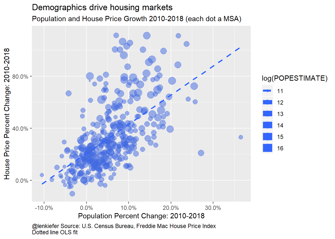
Figure 1: Population and House Price Growth 2010-2018
There’s a pretty strong association between nominal house price growth and population. The dotted line in the plot shows the Ordinary Least Squares (OLS) fit for the points.
stargazer::stargazer(lm(data=filter(df3, year==2018),
                        formula= I(hpi2010-1) ~ I(pop2010-1)), type="html",
                     covariate.labels = "Population Growth Rate: 2010-2018 (%)",
                     dep.var.labels   = "House Price Growth Rate: 2010-2018 (%)",
                     title            = "MSA House Prices and Population Growth: 2010-2018",
notes = "Source: U.S. Census 2018 Population Vintage Estimates, Freddie Mac House Price Index")| Dependent variable: | |
| House Price Growth Rate: 2010-2018 (%) | |
| Population Growth Rate: 2010-2018 (%) | 2.238*** |
| (0.156) | |
| Constant | 0.207*** |
| (0.013) | |
| Observations | 382 |
| R2 | 0.350 |
| Adjusted R2 | 0.348 |
| Residual Std. Error | 0.202 (df = 380) |
| F Statistic | 204.558*** (df = 1; 380) |
| Note: | p<0.1; p<0.05; p<0.01 |
| Source: U.S. Census 2018 Population Vintage Estimates, Freddie Mac House Price Index | |
The regression indicates that for every 1 percentage point increase in MSA population from 2010 to 2018 is associated with 2.2 percentage points higher house price growth.
How do the individual components of population growth correlate with house prices? Let’s take a look.
Let’s consider the association of house prices with migration, both domestic and international.
ggplot(data=filter(df3, CBSA %in% clist[1:25], year==2018), aes(x=domg,y=hpa))+
  geom_point(alpha=0.5, color="royalblue")+
  ggrepel::geom_text_repel( aes(label=NAME), color="royalblue", size=3)+
  scale_y_continuous(labels=percent)+
  scale_x_continuous(labels=percent)+
  theme(plot.caption=element_text(hjust=0))+
  stat_smooth(method="lm",fill=NA,linetype=2)+
  labs(x="Net Domestic Migration in 2018 as Percent of Population in 2017",
       y="House Price Percent Change 2017-2018",
       title="Demographics drive housing markets",
       subtitle="Net Domestic Migration and House Price Growth 2018 (each dot a MSA, top 25 by 2010 pop)",
       caption="@lenkiefer Source: U.S. Census Bureau, Freddie Mac House Price Index\nDotted line OLS fit")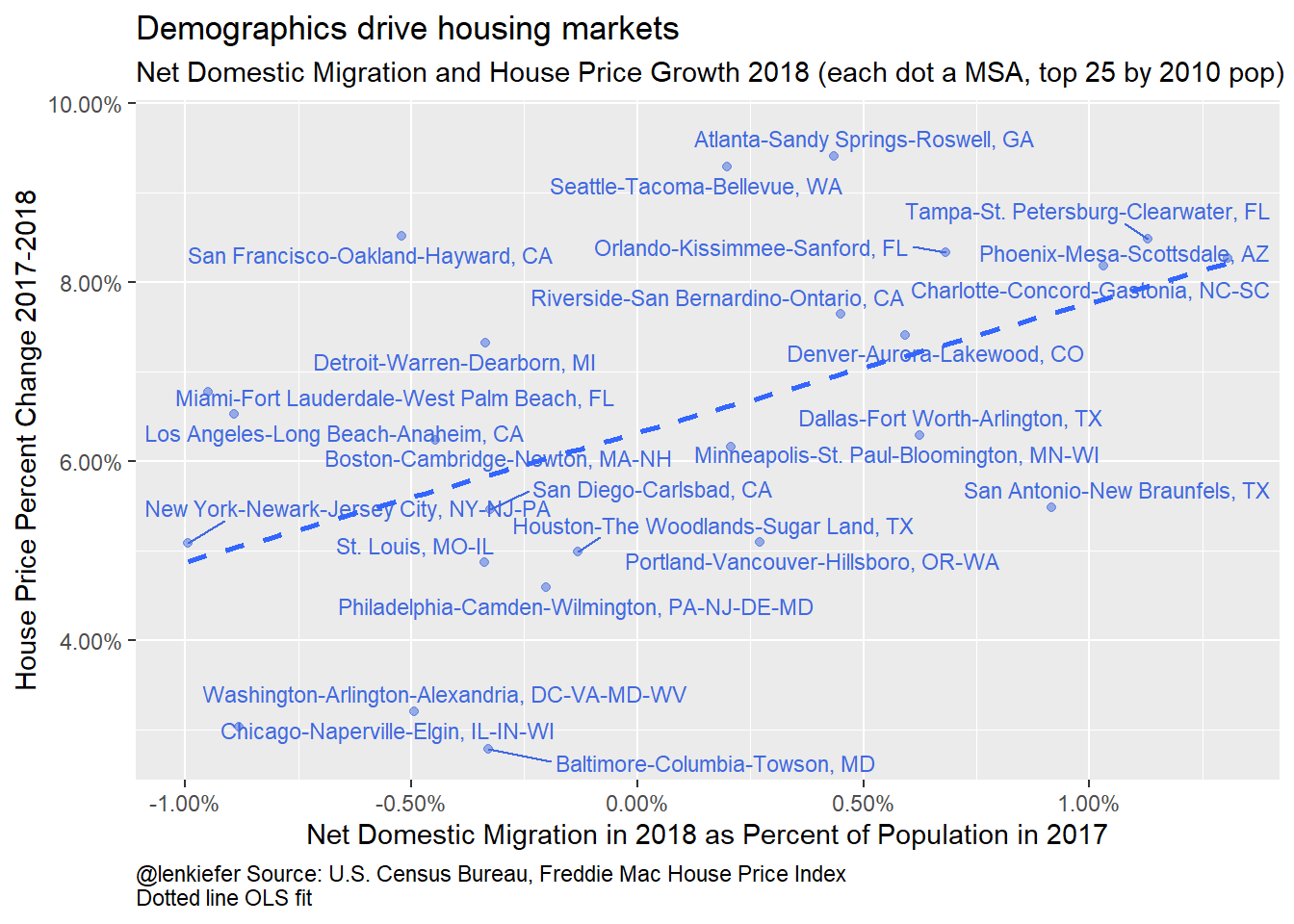
Figure 2: Domestic Migration and House Price Growth 2018
ggplot(data=filter(df3, year==2018), aes(x=domg,y=hpa))+
  geom_point(alpha=0.5, color="royalblue")+
  scale_y_continuous(labels=percent)+
  scale_x_continuous(labels=percent)+
  theme(plot.caption=element_text(hjust=0))+
  stat_smooth(fill=NA,linetype=2)+
  labs(x="Net Domestic Migration in 2018 as Percent of Population in 2017",
       y="House Price Percent Change 2017-2018",
       title="Demographics drive housing markets",
       subtitle="Net Domestic Migration and House Price Growth 2018 (each dot a MSA, all MSAs)",
       caption="@lenkiefer Source: U.S. Census Bureau, Freddie Mac House Price Index\nDotted lin LOESS fit")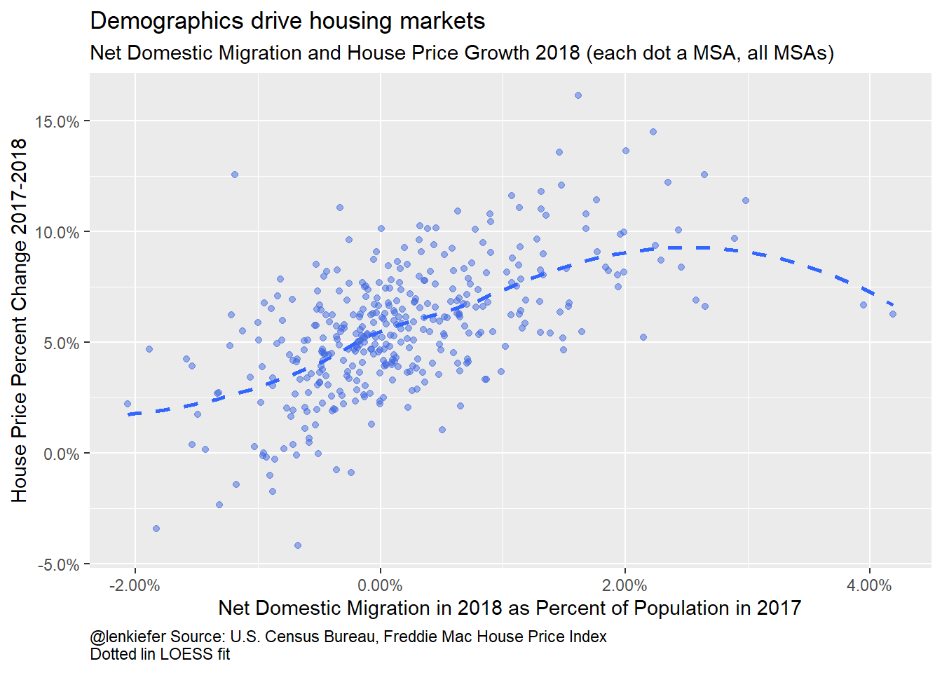
Figure 3: Domestic Migration and House Price Growth 2018
How about international migration?
ggplot(data=filter(df3, CBSA %in% clist[1:25], year==2018), aes(x=ig,y=hpa))+
  geom_point(alpha=0.5, color="royalblue")+
  ggrepel::geom_text_repel( aes(label=NAME), color="royalblue", size=3)+
  scale_y_continuous(labels=percent)+
  scale_x_continuous(labels=percent)+
  theme(plot.caption=element_text(hjust=0))+
  stat_smooth(method="lm",fill=NA,linetype=2)+
  labs(x="International Migration in 2018 as Percent of Population in 2017",
       y="House Price Percent Change 2017-2018",
       title="Demographics drive housing markets",
       subtitle="International Migration and House Price Growth 2018 (each dot a MSA, top 25 by 2010 pop)",
       caption="@lenkiefer Source: U.S. Census Bureau, Freddie Mac House Price Index\nDotted line OLS fit")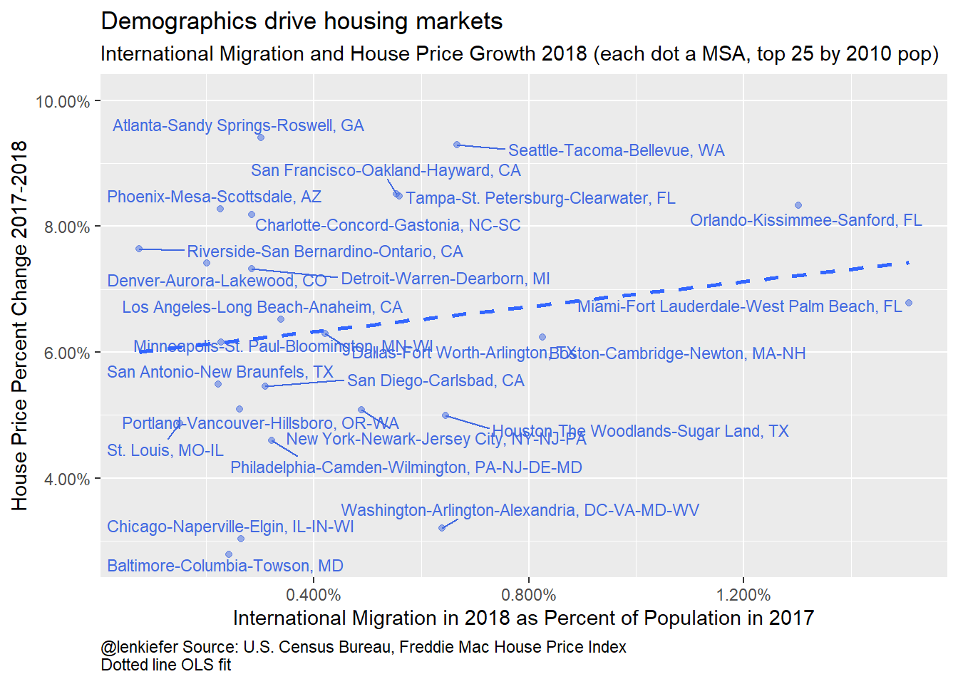
Figure 4: International Migration and House Price Growth 2018
ggplot(data=filter(df3, year==2018), aes(x=ig,y=hpa))+
  geom_point(alpha=0.5, color="royalblue")+
  scale_y_continuous(labels=percent)+
  scale_x_continuous(labels=percent)+
  theme(plot.caption=element_text(hjust=0))+
  stat_smooth(fill=NA,linetype=2)+
  labs(x="International Migration in 2018 as Percent of Population in 2017",
       y="House Price Percent Change 2017-2018",
       title="Demographics drive housing markets",
       subtitle="International Migration and House Price Growth 2018 (each dot a MSA, all MSAs)",
       caption="@lenkiefer Source: U.S. Census Bureau, Freddie Mac House Price Index\nDotted line LOESS fit")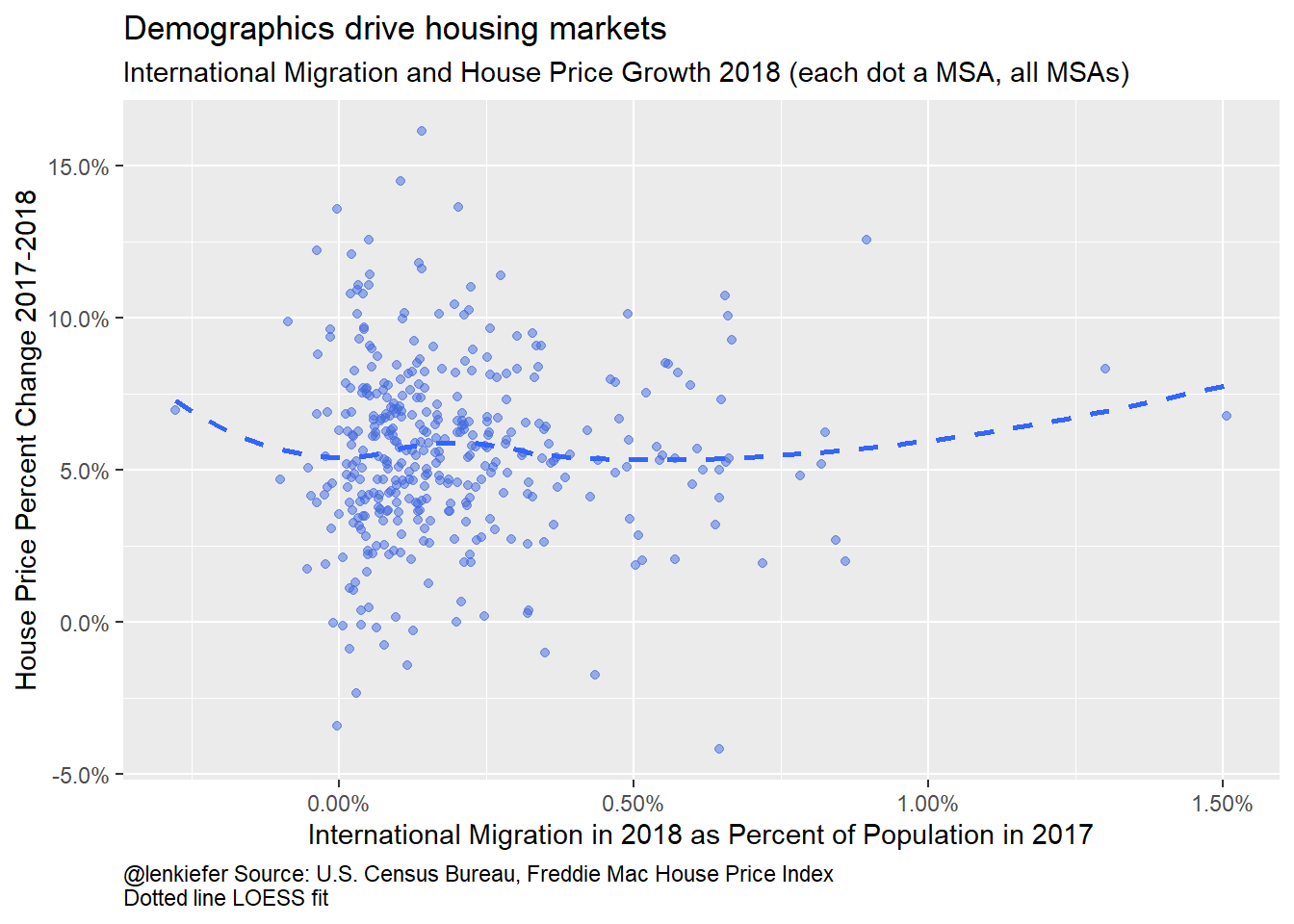
Figure 5: International Migration and House Price Growth 2018
And how about natural population growth (births minus deaths)?
ggplot(data=filter(df3, CBSA %in% clist[1:25], year==2018), aes(x=ng,y=hpa))+
  geom_point(alpha=0.5, color="royalblue")+
  ggrepel::geom_text_repel( aes(label=NAME), color="royalblue", size=3)+
  scale_y_continuous(labels=percent)+
  scale_x_continuous(labels=percent)+
  theme(plot.caption=element_text(hjust=0))+
  stat_smooth(method="lm",fill=NA,linetype=2)+
  labs(x="Natural Population Growth in 2018 as Percent of Population in 2017",
       y="House Price Percent Change 2017-2018",
       title="Demographics drive housing markets",
       subtitle="Natural Population Growth and House Price Growth 2018 (each dot a MSA, top 25 by 2010 pop)",
       caption="@lenkiefer Source: U.S. Census Bureau, Freddie Mac House Price Index\nDotted line OLS fit")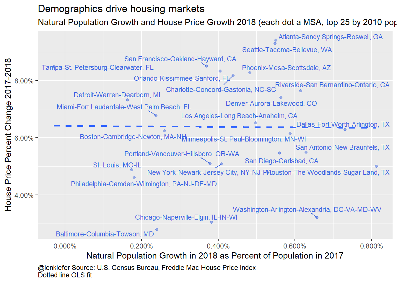
Figure 6: Natural Population Growth and House Price Growth 2018
ggplot(data=filter(df3, year==2018), aes(x=ng,y=hpa))+
  geom_point(alpha=0.5, color="royalblue")+
  #ggrepel::geom_text_repel( aes(label=NAME), color="royalblue", size=3)+
  scale_y_continuous(labels=percent)+
  scale_x_continuous(labels=percent)+
  theme(plot.caption=element_text(hjust=0))+
  stat_smooth(fill=NA,linetype=2)+
  labs(x="Natural Population Growth in 2018 as Percent of Population in 2017",
       y="House Price Percent Change 2017-2018",
       title="Demographics drive housing markets",
       subtitle="Natural Population Growth and House Price Growth 2018 (each dot a MSA, all MSAs)",
       caption="@lenkiefer Source: U.S. Census Bureau, Freddie Mac House Price Index\nDotted line LOESS fit")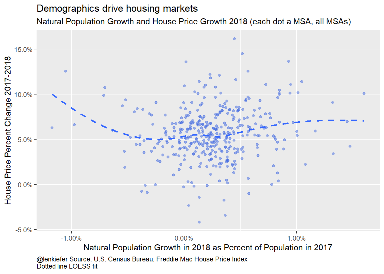
Figure 7: Natural Population Growth and House Price Growth 2018
The plots suggest that it’s domestic migration that’s the key component driving house prices in the short run. Let’s take a look by regressing metro house price growth on the components of population growth.
# regression results
stargazer::stargazer(lm(data=df3,
                        formula= hpa ~ ng+ig+domg+ I(factor(year))-1 ),
                     type="html",
                     title            = "MSA House Prices and Population Dynamics: 2010-2018",
          covariate.labels = c("Natural Population Growth Rate",
                               "International Migration Rate",
                               "Domestic Migration Rate",paste0("Year:", 2011:2018)),
          dep.var.labels   = "Annual House Price Growth Rate (%)",
notes = "Source: U.S. Census 2018 Population Vintage Estimates, Freddie Mac House Price Index")| Dependent variable: | |
| Annual House Price Growth Rate (%) | |
| Natural Population Growth Rate | 1.431*** |
| (0.153) | |
| International Migration Rate | 1.231*** |
| (0.299) | |
| Domestic Migration Rate | 1.910*** |
| (0.066) | |
| Year:2011 | -0.048*** |
| (0.002) | |
| Year:2012 | 0.003 |
| (0.002) | |
| Year:2013 | 0.053*** |
| (0.002) | |
| Year:2014 | 0.026*** |
| (0.002) | |
| Year:2015 | 0.032*** |
| (0.002) | |
| Year:2016 | 0.037*** |
| (0.002) | |
| Year:2017 | 0.044*** |
| (0.002) | |
| Year:2018 | 0.047*** |
| (0.002) | |
| Observations | 3,056 |
| R2 | 0.710 |
| Adjusted R2 | 0.709 |
| Residual Std. Error | 0.031 (df = 3045) |
| F Statistic | 677.654*** (df = 11; 3045) |
| Note: | p<0.1; p<0.05; p<0.01 |
| Source: U.S. Census 2018 Population Vintage Estimates, Freddie Mac House Price Index | |
These results indicate that about 70% of the cross sectional variation in MSA nominal house price growth rates from 2011-2018 can be explained by variations in the components of MSA population growth. Each percent increase in population due to natural populationg rowth is associated with 1.4 percent higher house price growth, each percent increase in international migration is associated with 1.2 percent higher house price growth, while one percent higher domestic migration is associated with 1.9 percent higher house price growth.
Let’s consider various models where we include either all population growth or the various components
# regression results
out1 <- lm(data=df3, formula= hpa ~ pg+ I(factor(year))-1 )
out2 <- lm(data=df3, formula= hpa ~ ng+ I(factor(year))-1 )
out3 <- lm(data=df3, formula= hpa ~ ig+ I(factor(year))-1 )
out4 <- lm(data=df3, formula= hpa ~ domg+ I(factor(year))-1 )
out5 <- lm(data=df3, formula= hpa ~ ng+ig+domg+ I(factor(year))-1 )
out6 <- lm(data=df3, formula= hpa ~  I(factor(year))-1 )


stargazer::stargazer(out1,out2,out3,out4, out5,out6,
                     type="html",
                     title            = "MSA House Prices and Population Dynamics: 2010-2018",
          covariate.labels = c("Population Growth Rate",
                               "Natural Population Growth Rate",
                               "International Migration Rate",
                               "Domestic Migration Rate",paste0("Year:", 2011:2018)),
          column.labels = c("Population Growth Only",
                            "Natural Population Only ",
                            "International Migration Only",
                            "Domestic Migration Only" ,
                            "All Components",
                            "Year fixed effects only"),
          dep.var.labels   = "Annual House Price Growth Rate (%)",
notes = "Source: U.S. Census 2018 Population Vintage Estimates, Freddie Mac House Price Index")| Dependent variable: | ||||||
| Annual House Price Growth Rate (%) | ||||||
| Population Growth Only | Natural Population Only | International Migration Only | Domestic Migration Only | All Components | Year fixed effects only | |
| (1) | (2) | (3) | (4) | (5) | (6) | |
| Population Growth Rate | 1.800*** | |||||
| (0.062) | ||||||
| Natural Population Growth Rate | 0.777*** | 1.431*** | ||||
| (0.164) | (0.153) | |||||
| International Migration Rate | 1.306*** | 1.231*** | ||||
| (0.327) | (0.299) | |||||
| Domestic Migration Rate | 1.767*** | 1.910*** | ||||
| (0.066) | (0.066) | |||||
| Year:2011 | -0.051*** | -0.043*** | -0.042*** | -0.040*** | -0.048*** | -0.039*** |
| (0.002) | (0.002) | (0.002) | (0.002) | (0.002) | (0.002) | |
| Year:2012 | 0.0002 | 0.009*** | 0.009*** | 0.011*** | 0.003 | 0.012*** |
| (0.002) | (0.002) | (0.002) | (0.002) | (0.002) | (0.002) | |
| Year:2013 | 0.051*** | 0.058*** | 0.059*** | 0.061*** | 0.053*** | 0.061*** |
| (0.002) | (0.002) | (0.002) | (0.002) | (0.002) | (0.002) | |
| Year:2014 | 0.023*** | 0.031*** | 0.032*** | 0.033*** | 0.026*** | 0.034*** |
| (0.002) | (0.002) | (0.002) | (0.002) | (0.002) | (0.002) | |
| Year:2015 | 0.030*** | 0.038*** | 0.038*** | 0.040*** | 0.032*** | 0.041*** |
| (0.002) | (0.002) | (0.002) | (0.002) | (0.002) | (0.002) | |
| Year:2016 | 0.035*** | 0.044*** | 0.043*** | 0.045*** | 0.037*** | 0.046*** |
| (0.002) | (0.002) | (0.002) | (0.002) | (0.002) | (0.002) | |
| Year:2017 | 0.042*** | 0.051*** | 0.051*** | 0.051*** | 0.044*** | 0.053*** |
| (0.002) | (0.002) | (0.002) | (0.002) | (0.002) | (0.002) | |
| Year:2018 | 0.045*** | 0.054*** | 0.054*** | 0.053*** | 0.047*** | 0.056*** |
| (0.002) | (0.002) | (0.002) | (0.002) | (0.002) | (0.002) | |
| Observations | 3,056 | 3,056 | 3,056 | 3,056 | 3,056 | 3,056 |
| R2 | 0.708 | 0.629 | 0.629 | 0.697 | 0.710 | 0.627 |
| Adjusted R2 | 0.707 | 0.628 | 0.628 | 0.697 | 0.709 | 0.626 |
| Residual Std. Error | 0.031 (df = 3047) | 0.035 (df = 3047) | 0.035 (df = 3047) | 0.032 (df = 3047) | 0.031 (df = 3045) | 0.035 (df = 3048) |
| F Statistic | 820.972*** (df = 9; 3047) | 575.055*** (df = 9; 3047) | 573.166*** (df = 9; 3047) | 780.283*** (df = 9; 3047) | 677.654*** (df = 11; 3045) | 639.669*** (df = 8; 3048) |
| Note: | p<0.1; p<0.05; p<0.01 | |||||
| Source: U.S. Census 2018 Population Vintage Estimates, Freddie Mac House Price Index | ||||||
The table has some interesting results. The last model (6) contains year only fixed effects and explains about 60% of the cross-MSA variation in house prices. If we add population controls we can explain an additional 10% or so of the cross sectional variation. Among the various components, domestic migration seems to do the best in predicting short-term house price movements.
This isn’t too surprising, as internal migration patterns likely reflect employment patterns. For example see my earlier post Employment growth and house price trends.
While these correlations are interesting, they should be interpreted with care. Migration patterns not only reflect shifting labor market trends but mostly likely are responding themselves to housing prices. Nevertheless these results underscore the importance of demographics for understanding house price movements.