House price gifski

I saw today, via Ropensci a blog post about a new package for making animated gifs with R called gifski now available on CRAN.

Let’s adapt the code we shared last week to use the gifski package. See that post for additional details.

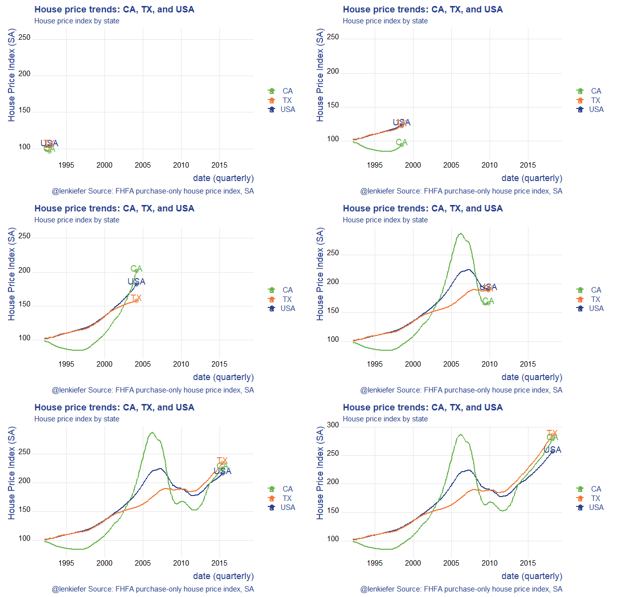
If we run the R code below we’ll generate this animated plot:

This plot shows the evolution of house prices in two states, California (CA) and Texas (TX) versus the United States (USA).

The new thing is that the code below swaps out the animation package saveGIF() call for gifski::save_gif. It seems gifski does save some time, though in this example the gains are relatively small. In future I’ll try it out with some of my more complex animations.

# load libraries ----
library(data.table)
library(gifski)
library(tweenr)
library(tidyverse)
library(lubridate)
library(tweenr)
library(ggridges)

# get house price data
df.hpi<-fread("https://www.fhfa.gov/DataTools/Downloads/Documents/HPI/HPI_master.csv")

df.hpi <- mutate(df.hpi,date=as.Date(ISOdate(yr,period*3,1)))

df.us <- filter(df.hpi, place_name=="United States", 
                hpi_type=="traditional",
                hpi_flavor=="purchase-only", 
                frequency=="quarterly")

df.state <- filter(df.hpi, level=="State",  
                   hpi_type=="traditional", 
                   hpi_flavor=="purchase-only", 
                   frequency=="quarterly")

df.stack <- bind_rows(df.us,df.state)


dfp <- 
  filter(df.stack,year(date)>1991) %>% 
  select(date,level,place_id,index_sa) %>%
  group_by(level,place_id) %>% 
  mutate(day=1+(row_number()-1), ease="linear", 
         rate_label=as.factor(as.character(round(index_sa,0)))) %>%
  ungroup() %>%
  mutate_if(is.character, as.factor)

# restrict to three plots
dfp2 <- filter(dfp, place_id %in% c("USA","TX","CA"))

dfp2 <- 
  dfp2 %>% 
  select(date,place_id,index_sa) %>% 
  spread(place_id,index_sa) %>%
  mutate(day=1+(row_number()-1), ease="linear")

# use tweener::tween_elements and tweener::tween_appear for a smooth interpolation between time points.
plot_data_tween<-
  tween_elements(dfp2,
                 time = "day",  group="ease",
                 ease="ease", nframes = nrow(dfp2)*3)

df_tween_appear <- tween_appear(plot_data_tween, time='day', nframes = nrow(dfp2)*3)
N <- max(df_tween_appear$.frame)

make_plot_appear <- function(i){
  p <-
    ggplot(data=df_tween_appear, aes(x=date,y=USA))+
    geom_line(alpha=0)+
    # code here is a bit dense, 
    geom_line(data=   .%>% filter(.frame==i, .age> -3.5) , aes(color="USA"),size=1.05) +
    geom_line(data=   .%>% filter(.frame==i, .age> -3.5) , aes(y=CA ,color=" CA"),size=1.05) +
    geom_line(data=   .%>% filter(.frame==i, .age> -3.5), aes(y=TX,color=" TX"),size=1.05 ) +
    geom_point(data=  .%>% filter(.frame==i, .age> -3.5) %>% tail(1), size=3, alpha=0.5, aes(color="USA"))+
    geom_point(data=  .%>% filter(.frame==i, .age> -3.5) %>% tail(1), size=3, alpha=0.5 , aes(y=CA ,color=" CA"))+
    geom_point(data=  .%>% filter(.frame==i, .age> -3.5) %>% tail(1),  size=3, alpha=0.5, aes(y=TX,color= " TX"))+
    geom_text(data=   .%>% filter(.frame==i, .age> -3.5) %>% tail(1), size=5, alpha=0.95, aes(label="USA",color="USA"),nudge_y=5)+
    geom_text(data=   .%>% filter(.frame==i, .age> -3.5) %>% tail(1),  size=5, alpha=0.95 , aes(y=CA ,label="CA",color=" CA"),nudge_y=5)+
    geom_text(data=   .%>% filter(.frame==i, .age> -3.5) %>% tail(1),  size=5, alpha=0.95, aes(y=TX,label="TX",color=" TX"),nudge_y=5)+
    theme_ridges(font_family="Roboto")+
    scale_color_manual(name="",values=c(rgb(103,180,75, maxColorValue = 256),"#f37735","#27408b"))+
    theme(text = element_text(color = "#27408b"))+
    labs(y="House Price Index (SA)",x="date (quarterly)",
         title="House price trends: CA, TX, and USA",
         subtitle="House price index by state",
         caption="@lenkiefer Source: FHFA purchase-only house price index, SA")
  
  return(p)
}

# to test plot, could run: 
# make_plot_appear(max(df_tween_appear$.frame))

# Set to your directory
mydir<-"YOURDIRECTORY"

t1 <-Sys.time()
gif_file <- save_gif({for (i in seq((1):N)){  
  g<- make_plot_appear(i)
  print(g)
  print(paste(i,"out of",N))
  }
  for (ii in 1:30){
    print(g)
    print(paste(ii,"out of",30))
  }
}, gif_file= paste0(mydir,"/hpa2.gif"),width = 620, height = 400, res = 92, delay=1/20)
t2 <- Sys.time()
t2-t1

Lots more to try with this!

 Share!

• Tweet