I think a lot about predicting/forecasting binary outcomes. Will the economy head into a recession next year? What’s the likelihood of a loan defaulting over the next few years? Will my followers on social media abandon me if I tweet about my lunch?
One often maligned, but seemingly irresitable approach to modeling binary ourcomes is the Linear Probability Model (LPM). As is known going back to before I was born, the Linear Probability Model has some issues. In particular, it is biased and inconsistent. But is it all that bad? Let’s take a look.
Here are a couple of handy references.
References
Amemiya, T. (1977). Some theorems in the linear probability model. International Economic Review, 645-650. JSTOR
Horrace, W. C., & Oaxaca, R. L. (2006). Results on the bias and inconsistency of ordinary least squares for the linear probability model. Economics Letters, 90(3), 321-327. pdf
Setup
We’re going to keep things simple here and follow the setup in Horrace and Oaxaca. We have a binary (0,1) outcome y that depends on a single regressor x.
The random variable \(x_i\beta\), our regressor times a coefficient falls in three intervals with the following probabilities:
\[ \begin{cases} PR(x_i\beta>1) = \pi,\\ PR(x_i\beta \in [0,1]) = \gamma,\\ PR(x_i\beta>1) = \rho \end{cases}\]
And the LPM is given by:
\[ \begin{cases} Pr(y_i =1 | x_i\beta>1) = 1, \\Pr(y_i=1|x_i\beta \in[0,1],= x_i\beta, \\Pr(y_i =1 | x_i\beta<0)=0 \end{cases}\]
Let’s draw a little picture using R.
library(tidyverse, quietly=T)
library(ggridges, quietly=T)
library(extrafont, quietly=T)
c0       <- 0  #intercept for process
beta_hat <- 0.4
gamma_hat <- pnorm((1-c0)/beta_hat) - pnorm(-c0/beta_hat)
rho_hat <- 1-pnorm((1-c0)/beta_hat)
pi_hat <- pnorm(-c0/beta_hat)


df <-
  data.frame(x=seq(-3,3,.01)) %>%
  mutate(p=pnorm(x/beta_hat+c0),
         shade=ifelse( beta_hat*x >= -1 & beta_hat*x <=1,p,NA))


  ggplot(data=df, aes(x=x,y=dnorm(x), fill="2gamma"))+
    geom_line(linetype=2)+
    geom_area(data= . %>% filter(beta_hat*x +c0 <=1, beta_hat*x + c0 >= 0), linetype=2,alpha=0.5)+
    scale_fill_manual(labels=c(expression(pi),expression(gamma),expression(rho)), name="region",
                      values=c(rgb(103,180,75, maxColorValue = 256),"#27408b","red"))+
    geom_area(data= . %>% filter(beta_hat*x + c0 <= 0), aes(y=dnorm(x), fill="1pi"), alpha=0.5)+
    geom_area(data= . %>% filter(beta_hat*x + c0 >= 1), aes(y=dnorm(x), fill="3rho"), alpha=0.5)+
    labs(x="X", y="Pr(X)", title="Likelihood of X",
         subtitle=expression(paste("Given ",beta," = 0.4")),
         caption=bquote(paste("Pr(",pi,")=",.(round(pi_hat,3)),
                              ", Pr(",gamma,")=",.(round(gamma_hat,3)),
                              ", Pr(",rho,")=",.(round(rho_hat,3)))))+
    theme_ridges(font_family="Roboto")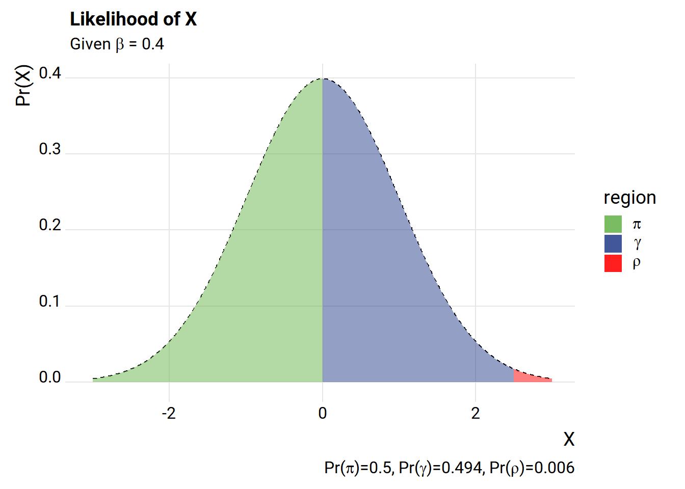
The way we’ve set it up, we have a very high likelihood of drawing an X value that is outside the \(\gamma\) range. Let’s add an intercept.
c0       <- 0.4  #intercept for process
beta_hat <- 0.4
gamma_hat <- pnorm((1-c0)/beta_hat) - pnorm(-c0/beta_hat)
rho_hat <- 1-pnorm((1-c0)/beta_hat)
pi_hat <- pnorm(-c0/beta_hat)


df <-
  data.frame(x=seq(-3,3,.01)) %>%
  mutate(p=pnorm(x/beta_hat+c0),
         shade=ifelse( beta_hat*x >= -1 & beta_hat*x <=1,p,NA))


  ggplot(data=df, aes(x=x,y=dnorm(x), fill="2gamma"))+
    geom_line(linetype=2)+
    geom_area(data= . %>% filter(beta_hat*x +c0 <=1, beta_hat*x + c0 >= 0), linetype=2,alpha=0.5)+
    scale_fill_manual(labels=c(expression(pi),expression(gamma),expression(rho)), name="region",
                      values=c(rgb(103,180,75, maxColorValue = 256),"#27408b","red"))+
    geom_area(data= . %>% filter(beta_hat*x + c0 <= 0), aes(y=dnorm(x), fill="1pi"), alpha=0.5)+
    geom_area(data= . %>% filter(beta_hat*x + c0 >= 1), aes(y=dnorm(x), fill="3rho"), alpha=0.5)+
    labs(x="X", y="Pr(X)", title="Likelihood of X",
         subtitle=expression(paste("Given ",beta," = 0.4, intercept=0.4")),
         caption=bquote(paste("Pr(",pi,")=",.(round(pi_hat,3)),
                              ", Pr(",gamma,")=",.(round(gamma_hat,3)),
                              ", Pr(",rho,")=",.(round(rho_hat,3)))))+
    theme_ridges(font_family="Roboto")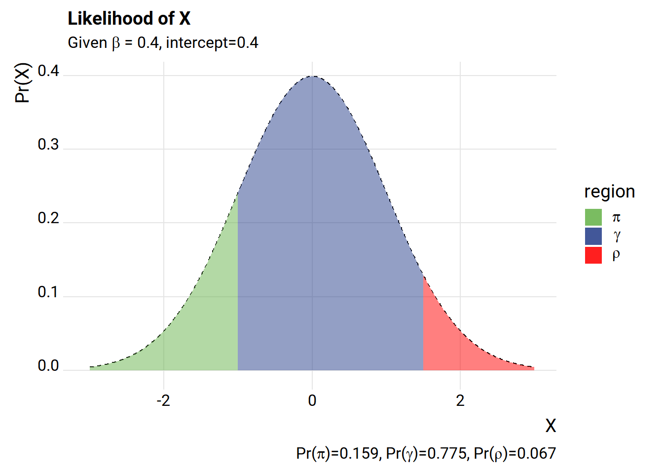
What happens if we simulate some data drawing from the process above and then estimate the LPM using Ordinary Least Squares (OLS)?
Simple simulation
  #helper function to truncate values at 0,1
 myf<- function(x){ case_when(
    x < 0  ~ 0,
    x >  1 ~ 1,
    TRUE ~ x)}

# Simulate under LPM
set.seed(180717)
c0       <- 0.4  #intercept for process
  beta_hat <- 0.4
  N <- 1000
  X <- rnorm(N)
  z <- c0+beta_hat*X
  Z0 <- myf(z)
  y <-  rbinom(N, size=1, prob=Z0)

  df.reg <- data.frame(y=y,x=X)
  summary(lm(data=df.reg, formula= y~x))
##
## Call:
## lm(formula = y ~ x, data = df.reg)
##
## Residuals:
## Min 1Q Median 3Q Max
## -0.85239 -0.31453 -0.01109 0.30487 0.85901
##
## Coefficients:
## Estimate Std. Error t value Pr(>|t|)
## (Intercept) 0.42063 0.01212 34.70 <2e-16 ***
## x 0.31511 0.01222 25.79 <2e-16 ***
## ---
## Signif. codes: 0 '***' 0.001 '**' 0.01 '*' 0.05 '.' 0.1 ' ' 1
##
## Residual standard error: 0.3833 on 998 degrees of freedom
## Multiple R-squared: 0.3999, Adjusted R-squared: 0.3993
## F-statistic: 665.1 on 1 and 998 DF, p-value: < 2.2e-16The true parameter values were 0.4 for both the intercept and the slope \(\beta\). Maybe we got a bad draw? Let’s simulate a number of draws.
We’ll create a helper function and use purrr::map and broom::tidy to help organize the results.
  myreg <- function(N=10){
    X <- rnorm(N)
    z <- c0+beta_hat*X
    Z0 <- myf(z)
    y <-  rbinom(N, size=1, prob=Z0)
    df.reg <- data.frame(y=y,x=X)
    broom::tidy(lm(data=df.reg, formula= y~x))
  }

# create samples of size 10, 100 and 1000, 1000 draws of  each

reg.df <- expand.grid(N=c(10,100,1000), trials=1:100)
suppressMessages(suppressWarnings(
reg.out <-
  reg.df  %>%
  mutate(lm=map(N,myreg)) %>%
  mutate(map(lm,broom::tidy)) %>%
  unnest(lm)   %>%
  select(N,trials,term,estimate)
))
#create summary table
reg.out %>%
  group_by(N,term) %>%
  summarize(ols.mean=mean(estimate),
            ols.median = median(estimate)) %>%
  mutate_if(is.numeric,round,3) %>%
  mutate(true.parameter=0.4) %>%
  arrange(term) %>%
htmlTable::htmlTable(caption="Mean/median over 100 trials of size N", css.cell = "padding-left: .5em; padding-right: .2em;", rnames=FALSE)| Mean/median over 100 trials of size N | ||||
| N | term | ols.mean | ols.median | true.parameter |
|---|---|---|---|---|
| 10 | (Intercept) | 0.418 | 0.41 | 0.4 |
| 100 | (Intercept) | 0.422 | 0.422 | 0.4 |
| 1000 | (Intercept) | 0.421 | 0.421 | 0.4 |
| 10 | x | 0.343 | 0.342 | 0.4 |
| 100 | x | 0.309 | 0.308 | 0.4 |
| 1000 | x | 0.311 | 0.311 | 0.4 |
Mean/median over 1,000 trials of size N
We see that the coefficients are quite biased, and as pointed out in Horrace and Oaxaca seem to get worse with larger sample size!
Trimming the estimates
Horrace and Oaxaca point out that trimming the estimates, removing observations when \(x_i\beta\) falls outside (0,1), may improve the estimates. Let’s give it a try.
# Function for trimmed estimates

  myreg.trim <- function(N=10){
    X <- rnorm(N)
    z <- c0+beta_hat*X
    Z0 <- myf(z)
    y <-  rbinom(N, size=1, prob=Z0)
    df.reg <- data.frame(y=y,x=X)
    #first stage
    out.lm <- lm(data=df.reg, formula= y~x)
    df.reg.trim <- df.reg[(predict(out.lm)>=0 & predict(out.lm)<=1 ),]
    out <-     broom::tidy(lm(data=df.reg.trim, formula= y~x))
    out$N.trim <- sum(predict(out.lm)>=0 & predict(out.lm)<=1 )
    return(out)
  }

 reg.df <- expand.grid(N=c(10,100,1000), trials=1:100)

suppressMessages(suppressWarnings(
  reg.out2 <- reg.df  %>%
    mutate(lm=map(N,myreg)) %>%
    mutate(map(lm,broom::tidy)) %>%
    mutate(lm.trim=map(N,myreg.trim)) %>%
    unnest(lm,lm.trim)   %>%
    select(N,trials,term,estimate, term1, estimate1)
))

reg.out2 %>% group_by(N,term) %>%
    summarize(ols.mean=mean(estimate),
              ols.median = median(estimate),
              trimmed.mean=mean(estimate1),
              trimmed.median = median(estimate1))%>%
  mutate(true.parameter=0.4) %>%
  mutate_if(is.numeric,round,3) %>%
  arrange(term) %>%
htmlTable::htmlTable(caption="Mean/median over 100 trials of size N", css.cell = "padding-left: .5em; padding-right: .2em;", rnames=FALSE)| Mean/median over 100 trials of size N | ||||||
| N | term | ols.mean | ols.median | trimmed.mean | trimmed.median | true.parameter |
|---|---|---|---|---|---|---|
| 10 | (Intercept) | 0.412 | 0.416 | 0.39 | 0.376 | 0.4 |
| 100 | (Intercept) | 0.419 | 0.421 | 0.398 | 0.395 | 0.4 |
| 1000 | (Intercept) | 0.422 | 0.422 | 0.405 | 0.406 | 0.4 |
| 10 | x | 0.321 | 0.318 | 0.483 | 0.439 | 0.4 |
| 100 | x | 0.311 | 0.308 | 0.384 | 0.38 | 0.4 |
| 1000 | x | 0.309 | 0.309 | 0.381 | 0.381 | 0.4 |
Seems to work a little better.
We’ll pick back up later with some additional analysis. In particular, I’m interested in studying how the bias changes given the distribution of X. If the likelihood of \(x_i\beta\) falling outside of the (0,1) range is zero, then the bias goes away. I’m also interested in looking at how aggregations over the LPM model behave.
Despite the defects in the LPM I still feel it has some strengths. Not only are the marginal effects more easily interpretable but it’s also easier to aggregate.
Are those advantages enough to overcome the disadvantages? That’s going to depend on the context. Next time we’ll explore some cases where it might be worthwhile.