Textmining is an exciting topic. There is tremendous potential to gain insights from textual analysis. See for example Gentzko, Kelly and Taddy’s Text as Data. While text mining may be quite advanced in other fields, in finance and economics the application of these techniques is still in its infancy.
In order to take advantage of text as data, economists and financial analysts need tools to help them. Fortunately, there is a great resource: Text Mining with R by Julia Silge (blog and on Twitter atjuliasilge) and David Robinson (blog and on Twitter atdrob). This text provides an excellent overview and examples using their tidytext package for R.
I was fortunate to have run into Julia at a R meetup in Salt Lake City a few weeks ago. Julia graciously shared some time with me and we talked about text mining. I left excited about applying tidytext principles to some applications.
Unfortunately I ran into a wall. I didn’t have data set up to get going. Many of the examples in Text Mining with R use already cleaned and organized data. This makes sense for their text so that they can demonstrate their powerful tools. But as is often the case, getting data ready for analysis was a significant barrier. But earlier this week a spark from across the internet re-ignited my interest in this topic.
In this post I want to share some experience I had applying the techniques in Text Mining with R (a joy!) and some of the strategies I used to begin to wrangle data in the wild into suitable form (not a joy!). We will look at a series of reports from the Board of Governors of the Federal Reserve and apply text mining techniques to them.
Wrangle
Once again the internet came through with an unexpected boon. In response to a tweet of mine on new home sales a user atisbrutussick shared a link to this post. In the post, the pdftools package was used to extract data from pdf files.
Yes! This is exactly what we need. We can use pdftools and a few other tricks to get the report data into R and in a form where we can start to apply tidytext tools.
Data format
The Federal Reserve is a natural target of text mining for economists. The Federal Open Market Committee (FOMC) monetary policy statement is parsed and prodded each time the FOMC announces a change (or no change at all). For example, the Wall Street Journal provides a Fed Statement Tracker which allows you to compare changes from one FOMC statement to another. Narasimhan Jegadeesh and Di Wu have a paper “Deciphering Fedspeak: The Information Content of FOMC Meetings” paper on ssrn that uses text mining techniques on FOMC meeting minutes.
Researchers have also looked at the transcripts for FOMC meetings. San Cannon has a paper “Sentiment of the FOMC Unscripted” pdf that applies text minging tools to FOMC transcripts.
We’ll look at the Federal Reserve’s semi-annual Monetary Policy Report. This report is typically issued in February and July, with the latest report for July 2018 released on July 13. We can download pdf files for each July report from 1996 through 2018, though the url form has changed slightly. The 2016 report was issued on June 21, 2016, but I’m going to label it July 2016 for consistency.
Import a single pdf
Let’s first load in a single report for July 2018 available at https://www.federalreserve.gov/monetarypolicy/files/20180713_mprfullreport.pdf.
We’ll need several libraries, which can all be downloaded from CRAN by running install.packages("packagename").
# load libraries ----
suppressPackageStartupMessages({
library(extrafont)
library(ggraph)
library(ggridges)
library(pdftools)
library(tidyverse)
library(tidytext)
library(forcats)
library(reshape2)
library(tidyr)
library(igraph)
library(widyr)
library(viridis)}

)
We’ll use pdftools to import the pdf file.
fed_import1 <- pdf_text("https://www.federalreserve.gov/monetarypolicy/files/20180713_mprfullreport.pdf")
str(fed_import1)
## chr [1:71] "" "" ...Uh oh. We’ve downloaded the pdf file as a a list of strings, one for each page (there are 71 pages in the report).
Let’s take a look at page 7’s first 500 characters.
substr(fed_import1[7],1,500)## [1] " 1\r\nSummary\r\nEconomic activity increased at a solid pace a sizable increase in consumer energy prices.\r\nover the first half of 2018, and the labor The 12-month measure of inflation that\r\nmarket has continued to strengthen. Inflation excludes food and energy items (so-called core\r\nhas moved up, and in May, the most recent inflation), which historically has been a better\r\nperiod for whi"Oh yuck! We’ve got a bunch of spaces and special characters \r and \n indicating linebreaks.
We can deal with this by splitting on \r with strsplit() and removing \n with gsub(). I have to look up regular expression every time I use them.
fed_text_raw <-
  data.frame(text=unlist(strsplit(fed_import1,"\r"))) %>%
  mutate(report="July2018",
         line=row_number(),
         text=gsub("\n","",text))
head(fed_text_raw)
## text report line
## 1 Letter of Transmittal July2018 1
## 2 Board of Governors of the July2018 2
## 3 Federal Reserve System July2018 3
## 4 Washington, D.C., July 13, 2018 July2018 4
## 5 The President of the Senate July2018 5
## 6 The Speaker of the House of Representatives July2018 6Now we’re about ready to rock!
Data Note
We still have a lot of filler like Letters of Transmittal, appendices with acronyms and other superfluous material. Unfortunately removing them requires examination of the document (front matter is different length in different reports). For today, we’ll ignore this and save more careful wrangling for future.
Text mining
Now we can begin to apply the tidytext mining technqiues outlined in Text Mining with R. I took these data and walked pretty much step by step through the book and learned a lot. Let me share some highlights.
fed_text <-
  fed_text_raw %>%
  as_tibble() %>%
  unnest_tokens(word,text)
fed_text
## # A tibble: 30,264 x 3
## report line word
## <chr> <int> <chr>
## 1 July2018 1 letter
## 2 July2018 1 of
## 3 July2018 1 transmittal
## 4 July2018 2 board
## 5 July2018 2 of
## 6 July2018 2 governors
## 7 July2018 2 of
## 8 July2018 2 the
## 9 July2018 3 federal
## 10 July2018 3 reserve
## # ... with 30,254 more rowsLet’s count up words:
fed_text  %>%
  count(word, sort = TRUE)
## # A tibble: 3,030 x 2
## word n
## <chr> <int>
## 1 the 2036
## 2 of 1174
## 3 in 778
## 4 and 725
## 5 to 525
## 6 for 407
## 7 rate 309
## 8 a 287
## 9 federal 268
## 10 on 230
## # ... with 3,020 more rowsOops! We have a lot of common words like “the”,“of”,and “in”. In text mining these words are called “stop words”. We can remove them by using anti-join and the stop_words list that comes in tidytext package.
fed_text  %>%
  anti_join(stop_words)%>%
  count(word, sort = TRUE)
## Joining, by = "word"## # A tibble: 2,653 x 2
## word n
## <chr> <int>
## 1 rate 309
## 2 federal 268
## 3 2018 229
## 4 policy 206
## 5 percent 188
## 6 projections 168
## 7 economic 161
## 8 2 157
## 9 inflation 154
## 10 monetary 141
## # ... with 2,643 more rowsGetting better! The Fed sures does like to talk about rates. But we also have some numbers in the text. The year 2018 appears a lot. And the number 2, associated with the Fed’s 2 percent inflation target, shows up a lot.
Let’s drop numbers from the text. In older reports, they liked to use fractions with special characters, so we’ll take a heavy-handed approach and only keep alphabetic characters.
fed_text2 <-
  fed_text %>%
  mutate(word = gsub("[^A-Za-z ]","",word)) %>%
  filter(word != "")

fed_text2  %>%
  anti_join(stop_words)%>%
  count(word, sort = TRUE)
## Joining, by = "word"## # A tibble: 2,323 x 2
## word n
## <chr> <int>
## 1 rate 309
## 2 federal 268
## 3 policy 206
## 4 percent 188
## 5 projections 168
## 6 economic 161
## 7 inflation 155
## 8 monetary 141
## 9 funds 132
## 10 participants 129
## # ... with 2,313 more rowsWhat’s the overall sentiment of the report? Text mining allows us to try to score text, or portions of text for sentiment. We can apply one of the sentiments datasets supplied by tidytext to score the report. For right now we’ll use the bing library based on Bing Liu and collaborators
Let’s see what the most frequently used negative and positive words are based on the bing lexicon.
fed_text2 %>%
  inner_join(get_sentiments("bing")) %>%
    count(word, sentiment, sort = TRUE)
## Joining, by = "word"## # A tibble: 239 x 3
## word sentiment n
## <chr> <chr> <int>
## 1 risks negative 50
## 2 appropriate positive 39
## 3 confidence positive 37
## 4 debt negative 26
## 5 strong positive 25
## 6 balanced positive 24
## 7 gross negative 24
## 8 decline negative 23
## 9 errors negative 23
## 10 well positive 23
## # ... with 229 more rowsSo risks a negative word is used 50 times in the report. Appropriate, a positive word, is used 39. But hey! Wait a second.
Debt is the fourth most frequent word in the list, considered negative. But in a economic report debt might be more descriptive than positive/negative.
Also, “gross” is probably associated with “Gross Domestic Product” rather than expressions of disgust. Let’s investigate.
ewww gross! exploring with bigrams
We can apply tidytext principles to single words, like above. But we can also apply them to consecutive sequences of words, called n-grams. Two words together are called bigrams.
fed_bigrams <-
  fed_text_raw %>%
  unnest_tokens(bigram, text, token = "ngrams", n = 2) %>%
  as_tibble()

fed_bigrams
## # A tibble: 27,533 x 3
## report line bigram
## <chr> <int> <chr>
## 1 July2018 1 letter of
## 2 July2018 1 of transmittal
## 3 July2018 2 board of
## 4 July2018 2 of governors
## 5 July2018 2 governors of
## 6 July2018 2 of the
## 7 July2018 3 federal reserve
## 8 July2018 3 reserve system
## 9 July2018 4 washington d.c
## 10 July2018 4 d.c july
## # ... with 27,523 more rowsNow we can count up bigrams:
fed_bigrams %>%
  count(bigram, sort = TRUE)
## # A tibble: 13,458 x 2
## bigram n
## <chr> <int>
## 1 <NA> 603
## 2 of the 308
## 3 in the 259
## 4 the federal 171
## 5 monetary policy 115
## 6 federal funds 109
## 7 funds rate 106
## 8 for the 100
## 9 federal reserve 79
## 10 to the 76
## # ... with 13,448 more rowsAs Silge and Robinson point out, many of these bigrams are uninteresing. Let’s filter out uninteresing bigrams that contain stop words.
bigrams_separated <- fed_bigrams %>%
  separate(bigram, c("word1", "word2"), sep = " ")

bigrams_filtered <- bigrams_separated %>%
  filter(!word1 %in% stop_words$word) %>%
  filter(!word2 %in% stop_words$word)

bigram_counts <- bigrams_filtered %>%
  count(word1, word2, sort = TRUE)

bigram_counts
## # A tibble: 4,662 x 3
## word1 word2 n
## <chr> <chr> <int>
## 1 <NA> <NA> 603
## 2 monetary policy 115
## 3 federal funds 109
## 4 funds rate 106
## 5 federal reserve 79
## 6 2 percent 46
## 7 unemployment rate 46
## 8 labor force 43
## 9 target range 40
## 10 prime age 36
## # ... with 4,652 more rows# unite them
bigrams_united <- bigrams_filtered %>%
unite(bigram, word1, word2, sep = " ")
bigrams_united## # A tibble: 9,366 x 3
## report line bigram
## <chr> <int> <chr>
## 1 July2018 3 federal reserve
## 2 July2018 3 reserve system
## 3 July2018 4 washington d.c
## 4 July2018 4 d.c july
## 5 July2018 4 july 13
## 6 July2018 4 13 2018
## 7 July2018 7 monetary policy
## 8 July2018 7 policy report
## 9 July2018 7 report pursuant
## 10 July2018 8 section 2b
## # ... with 9,356 more rowsNow let’s find out if the Fed got grossed out and disgusted by something, or as I suspect they were talking GDP most of the time when they used the word “gross”.
bigrams_filtered %>%
  filter(word1 == "gross") %>%
  count( word2, sort = TRUE)
## # A tibble: 5 x 2
## word2 n
## <chr> <int>
## 1 domestic 18
## 2 federal 1
## 3 gdp 1
## 4 issuance 1
## 5 real 1Yep, we’ll probably want to drop terms like “gross” from the sentiment score.
Revised sentiment
I analyzed the report word frequencies and came up with a list of words that probably aren’t negative in the usual sense. The word “crude” for example is associated with oil.
There’s another lexicon “loughran” that’s more tuned to financials, but as discussed in Cannon (2015), this lexicon might be too restrictive for Fedspeak.
Instead I took the bing list and added some custom words. We can bind a list of custom words to our stop_words dataset and filter. Following Silge and Robinson we can use the %/% operator to break the text up into 80 line sections (about 3 pages of text).
custom_stop_words2 <-
  bind_rows(data_frame(word = c("debt",
                                "gross",
                                "crude",
                                "well",
                                "maturity",
                                "work",
                                "marginally",
                                "leverage"),
                       lexicon = c("custom")),
            stop_words)


fed_sentiment <-
  fed_text %>%
  anti_join(custom_stop_words2) %>%
  inner_join(get_sentiments("bing")) %>%
  count(report, index = line %/% 80, sentiment) %>%
  spread(sentiment, n, fill = 0) %>%
  mutate(sentiment = positive - negative)
## Joining, by = "word"
## Joining, by = "word"ggplot(fed_sentiment, aes(index, sentiment, fill = sentiment>0)) +
geom_col(show.legend = FALSE) +
scale_fill_manual(values=c("red","#27408b"))+
facet_wrap(~report, ncol = 5, scales = "free_x")+
theme_ridges(font_family="Roboto")+
labs(x="index (approximately 3 pages per unit)",y="sentiment",
title="Sentiment through Federal Reserve Monetary Policy Report",
subtitle="customized bing lexicon",
caption="@lenkiefer\nSource: https://www.federalreserve.gov/monetarypolicy/files/20180713_mprfullreport.pdf")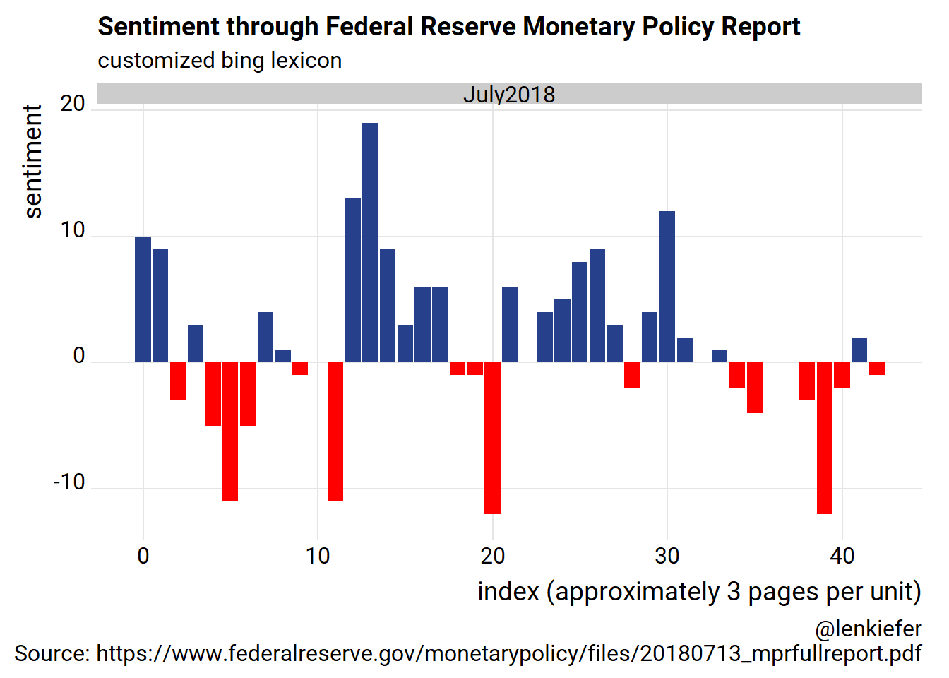
This trend tell an interesting story. The text began positive, dropped off but then surged in the middle. Around the last third of the text, near part 3: Summary of Economic Projections sentiment turns negative as the text describes forecasts and risks.
Comparing multiple reports
Let’s expand our analysis by capturing the text of each Monetary Policy Report for July from 1996 through 2018. We’ll compare the relative frequency of words and topics and see how sentiment (as we captured it above) varies across reports. The 2016 report was issued on June 21, 2016, but I’m going to label it July 2016 for consistency.
Unfortunately the links to the various reports follow a changing pattern, but fortunately for you I have gone and found the URL for each July report. The following code will collect the pdf files and get it ready for tidytext mining.
# list of reports, comments indicate important events around release of report
fed.links=c("https://www.federalreserve.gov/monetarypolicy/files/20180713_mprfullreport.pdf",
            "https://www.federalreserve.gov/monetarypolicy/files/20170707_mprfullreport.pdf",
            "https://www.federalreserve.gov/monetarypolicy/files/20160621_mprfullreport.pdf",            # released in jun 2016, but we'll label it July
            "https://www.federalreserve.gov/monetarypolicy/files/20150715_mprfullreport.pdf",            # July 2015  ( before lift off)
            "https://www.federalreserve.gov/monetarypolicy/files/20140715_mprfullreport.pdf",
            "https://www.federalreserve.gov/monetarypolicy/files/20130717_mprfullreport.pdf",            # July 2013  ( after Taper Tantrum)
            "https://www.federalreserve.gov/monetarypolicy/files/20120717_mprfullreport.pdf",
            "https://www.federalreserve.gov/monetarypolicy/files/20110713_mprfullreport.pdf",            # July 2011  ( early recovery)
            "https://www.federalreserve.gov/monetarypolicy/files/20100721_mprfullreport.pdf",
            "https://www.federalreserve.gov/monetarypolicy/files/20090721_mprfullreport.pdf",            # July 2009  ( end of Great Recession)
            "https://www.federalreserve.gov/monetarypolicy/files/20080715_mprfullreport.pdf",
            "https://www.federalreserve.gov/monetarypolicy/files/20070718_mprfullreport.pdf" ,           # July 2007  ( eve of  Great Recession)
            "https://www.federalreserve.gov/boarddocs/hh/2006/july/fullreport.pdf",
            "https://www.federalreserve.gov/boarddocs/hh/2005/july/fullreport.pdf",                      # July 2005  ( housing boom)
            "https://www.federalreserve.gov/boarddocs/hh/2004/july/fullreport.pdf",
            "https://www.federalreserve.gov/boarddocs/hh/2003/july/FullReport.pdf" ,                     # July 2003  ( deflation fears)
            "https://www.federalreserve.gov/boarddocs/hh/2002/july/FullReport.pdf",
            "https://www.federalreserve.gov/boarddocs/hh/2001/july/FullReport.pdf",                      # July 2001  ( dot come Recession)
            "https://www.federalreserve.gov/boarddocs/hh/2000/July/FullReport.pdf",
            "https://www.federalreserve.gov/boarddocs/hh/1999/July/FullReport.pdf",                      # July 1999  ( eve of dotcom Recession)
            "https://www.federalreserve.gov/boarddocs/hh/1998/july/FullReport.pdf",
            "https://www.federalreserve.gov/boarddocs/hh/1997/july/FullReport.pdf",                       # July 1997 ( irrational exhuberance)
            "https://www.federalreserve.gov/boarddocs/hh/1996/july/FullReport.pdf"
            )


df_fed <-
  data.frame(report=c("Jul2018",paste0("Jul",seq(2017,1996,-1))),stringsAsFactors = FALSE) %>%
  mutate(text= map(fed.links,pdf_text)) %>% unnest(text) %>%
  group_by(report) %>% mutate(page=row_number()) %>%
  ungroup() %>% mutate(text=strsplit(text,"\r")) %>% unnest(text) %>% mutate(text=gsub("\n","",text)) %>%
  group_by(report) %>% mutate(line=row_number()) %>% ungroup() %>% select(report,line,page,text)
Basic text statistics
Let’s see what we have by computing some basic text statistics.
Compare word counts
Let’s start with just the number of words per report.
fed_words <- df_fed %>%
  unnest_tokens(word, text) %>%
  count(report, word, sort = TRUE) %>%
  ungroup()

total_words <- fed_words %>%
  group_by(report) %>%
  summarize(total = sum(n))

# total words per report

ggplot(data=total_words, aes(x=seq(1996,2018),y=total))+
  geom_line(color="#27408b")+
  geom_point(shape=21,fill="white",color="#27408b",size=3,stroke=1.1)+
  scale_y_continuous(labels=scales::comma)+
  theme_ridges(font_family="Roboto")+
  labs(x="year",y="number of words",
       title="Number of words in Federal Reserve Monetary Policy Report",
       subtitle="July of each year 1996-2018",
       caption="@lenkiefer Source: Federal Reserve Board Monetary Policy Reports")
So the 2018 report at over 30,000 words is one of the longer reports. We also can see a pretty clear break at the end of the Greenspan tenure in 2005 as the reports got substantially longer.
What were they talking about?
Let’s compile a list of most frequently used words in each report. As before, we’ll omit stop words.
fed_text <-
  df_fed %>%
  select(report,page,line,text) %>%
  unnest_tokens(word,text)

fed_text %>%
  mutate(word = gsub("[^A-Za-z ]","",word)) %>%  # keep only letters (drop numbers and special symbols)
  filter(word != "") %>%
  anti_join(stop_words) %>%
  group_by(report) %>%
  count(word,sort=TRUE) %>%
  mutate(rank=row_number()) %>%
  ungroup() %>%
  arrange(rank,report) %>%
  filter(rank<11) %>%
  ggplot(aes(y=n,x=fct_reorder(word,n))) +
  geom_col(fill="#27408b")+
  facet_wrap(~report,scales="free", ncol=5)+
  coord_flip()+
  theme_ridges(font_family="Roboto", font_size=10)+
  labs(x="",y="",
       title="Most Frequent Words Federal Reserve Monetary Policy Report",
       subtitle="Excluding stop words and numbers.",
       caption="@lenkiefer Source: Federal Reserve Board Monetary Policy Reports")
## Joining, by = "word"
Lots of talking about rates. Let’s see if we can get something more informative out of these data.
Following Silge and Robinson we can use the bind_tf_idf function to bind the term frequency and inverse document frequency to our tidy text dataset. This statistic will decrease the weight on very common words and increase the weight on words that only appear in a few documents. In essence, we extract what’s special about each report. The Monetary Policy Report is always going to talk a lot about interest rates and the general economy, but the tf-idf statistic can tell us something about what’s different in each report.
We’ll also clean out some additional terms that the pdftools picked up (like month abberviations) by augmenting our stop word list. This list also include word fragments like ‘ing’ that result from words spanning columns.
# Custom stop words
custom_stop_words <-
  bind_rows(data_frame(word = c(tolower(month.abb), "one","two","three","four","five","six",
                                "seven","eight","nine","ten","eleven","twelve","mam","ered",
                                "produc","ing","quar","ters","sug","quar",'fmam',"sug",
                                "cient","thirty","pter",
                                "pants","ter","ening","ances","www.federalreserve.gov",
                                "tion","fig","ure","figure","src"),
                       lexicon = c("custom")),
            stop_words)


fed_textb <-
  fed_text %>%

  mutate(word = gsub("[^A-Za-z ]","",word)) %>%  # keep only letters (drop numbers and special symbols)
  filter(word != "") %>%
  count(report,word,sort=TRUE) %>%
  bind_tf_idf(word, report, n) %>%
  arrange(desc(tf_idf))

fed_textb %>%
    anti_join(custom_stop_words, by="word") %>%
  mutate(word = factor(word, levels = rev(unique(word)))) %>%
  group_by(report) %>%
  mutate(id=row_number()) %>%
  ungroup() %>%
  filter(id<11) %>%
  ggplot(aes(word, tf_idf, fill = report)) +
  geom_col(show.legend = FALSE) +
  labs(x = NULL, y = "tf-idf") +
  facet_wrap(~report,scales="free", ncol=5)+
  coord_flip()+
  theme_ridges(font_family="Roboto", font_size=10)+
  theme(axis.text.x=element_blank())+
  labs(x="",y ="tf-idf",
       title="Highest tf-idf words in each Federal Reserve Monetary Policy Report: 1996-2018",
       subtitle="Top 10 terms by tf-idf statistic: term frequncy and inverse document frequency",
       caption="@lenkiefer Source: Federal Reserve Board Monetary Policy Reports\nNote: omits stop words, date abbreviations and numbers.")
This chart tells a fascinating story. We can see the emergence of certain acronyms like JGTRRA (Jobs and Growth Tax Relief Reconciliation Act), TALF (Term Asset-Basked Securities Loan Facility) or lfpr (labor force participation rate). You can also see terms such as terrorism (2002) and war (2003) associated with major geopolitical events.
The Monetary Policy Report also often contains a special topic, and you can see signs of them in some of the reports. For example, the 2016 report had a special topic: “Have the Gains of the Economic Expansion Been Widely Shared?” that discussed economic trends across demographic groups. You can see evidence of that with the prevalence of terms like “hispanic”,“race”,“black”, and “white” in the 2016 report.
Comparing sentiment across reports
How did sentiment vary across reports? Let’s use the approach we used above for the 2018 report and apply it to each report.
fed_sentiment <-
  fed_text %>%
  anti_join(custom_stop_words2) %>%
  inner_join(get_sentiments("bing")) %>%
  count(report, index = line %/% 80, sentiment) %>%
  spread(sentiment, n, fill = 0) %>%
  mutate(sentiment = positive - negative)
## Joining, by = "word"
## Joining, by = "word"ggplot(fed_sentiment, aes(index, sentiment, fill = sentiment>0)) +
geom_col(show.legend = FALSE) +
scale_fill_manual(values=c("red","#27408b"))+
facet_wrap(~report, ncol = 5, scales = "free_x")+
theme_ridges(font_family="Roboto")+
labs(x="index (approximately 3 pages per unit)",y="sentiment",
title="Sentiment through Federal Reserve Monetary Policy Report",
subtitle="customized bing lexicon",
caption="@lenkiefer Source: Federal Reserve Board Monetary Policy Reports")
This result shows that sentiment tended to be negative in 2001-2003 and 2008-2009, which were right around the last two recessions.
Let’s compute total sentiment by report.
fed_sentiment2 <-
  fed_text %>%
  anti_join(custom_stop_words2) %>%
  inner_join(get_sentiments("bing")) %>%
  count(report, sentiment) %>%
  spread(sentiment, n, fill = 0) %>%
  mutate(sentiment = positive - negative)
## Joining, by = "word"
## Joining, by = "word"ggplot(fed_sentiment2, aes(factor(1996:2018), sentiment/(negative+positive), fill = sentiment)) +
geom_col(show.legend = FALSE) +scale_fill_viridis_c(option="C")+
theme_ridges(font_family="Roboto",font_size=10)+
labs(x="report for July of each year",y="Sentiment (>0 positive, <0 negtaive)",
title="Sentiment of Federal Reserve Monetary Policy Report: 1996-2018",
subtitle="customized bing lexicon",
caption="@lenkiefer Source: Federal Reserve Board Monetary Policy Reports")
Visualizing word correlations
We can follow Silge and Robinson and construct a graph to visualize word correlations and clusters of words. We’ll compute pairwise word correlations and then construct a graph using ggraph to represent those correlations. See section 4.2 of theText Mining with R as this follows precisly what’s presented there.
word_cors <-
  fed_text2 %>%
  mutate(section = row_number() %/% 10) %>%
  filter(section > 0) %>%
  filter(!word %in% stop_words$word) %>%
  group_by(word) %>%
  filter(n() >= 20) %>%
  pairwise_cor(word, section, sort = TRUE)

word_cors %>%
  filter(correlation > .15) %>%
  graph_from_data_frame() %>%
  ggraph(layout = "fr") +
  geom_edge_link(aes(edge_alpha = correlation), show.legend = FALSE) +
  geom_node_point(color ="#27408b", size = 5) +
  geom_node_text(aes(label = name), repel = TRUE) +
  theme_void(base_family="Roboto")+
  labs(title="  Pairs of words in Federal Reserve Monetary Policy Reports that show at\n  least a 0.15 correlation of appearing within the same 10-line section", caption="  @lenkiefer Source: July Federal Reserve Board Monetary Policy Reports 1996-2018    \n")
Conclusion
That’s all for today. I’m continuing to explore these techniques. So far I find them quite promising. In near future I’d like to explore Topic Modeling and other text mining techniques. On the front end, there’s still some additional work to do on the data wrangling front. I’ve added a new tag for textmining where you’ll see additional posts as I explore text mining.
References
Cannon, S. (2015). Sentiment of the FOMC: Unscripted. Economic Review-Federal Reserve Bank of Kansas City, 5. pdf
Gentzkow, M., Kelly, B. T., & Taddy, M. (2017). Text as data (No. w23276). National Bureau of Economic Research. pdf
Jegadeesh, N., & Wu, D. A. (2017). Deciphering fedspeak: The information content of fomc meetings. paper on ssrn
Silge, J., & Robinson, D. (2016). tidytext: Text mining and analysis using tidy data principles in r. The Journal of Open Source Software, 1(3), 37.
Silge, J., & Robinson, D. (2017). Text mining with R: A tidy approach. " O’Reilly Media, Inc.“. ebook, O’Reilly