LET’S PIXELATE AMERICA. This morning I happened across a fun blog post on how to generate Pixel maps with R via R weekly.
The basic code is so easy, all you need is ggplot2 (which I get from the tidyverse).
library(tidyverse)## Warning: package 'tidyverse' was built under R version 3.5.1## -- Attaching packages -------------------------------------------------------------------------------------------------------------------------------------------------------------------------------- tidyverse 1.2.1 --## v ggplot2 3.0.0 v purrr 0.2.5
## v tibble 1.4.2 v dplyr 0.7.6
## v tidyr 0.8.0 v stringr 1.3.1
## v readr 1.1.1 v forcats 0.3.0## Warning: package 'purrr' was built under R version 3.5.1## Warning: package 'stringr' was built under R version 3.5.1## -- Conflicts ----------------------------------------------------------------------------------------------------------------------------------------------------------------------------------- tidyverse_conflicts() --
## x dplyr::filter() masks stats::filter()
## x dplyr::lag() masks stats::lag()ggplot(map_data("state"), aes(round(long, 0),round(lat,0),
group=group, fill = as.factor(group))) +
geom_polygon() +
guides(fill=FALSE) +
coord_map() +
theme_void()##
## Attaching package: 'maps'## The following object is masked from 'package:purrr':
##
## map![]()
We can modify our dark theme and generate a dark background. Then we’ll animate it to get:
![]()
Using this code:
library(ggthemes)
library(animation)
library(tweenr)
library(extrafont)
library(gridExtra)
library(tidyr)  # for map function

 #  Function for use with tweenr
  myf<-function (d=6){
    d.out<-map.df
    d.out$lat<-round(d.out$lat,d) # round lat and lon
    d.out$long<-round(d.out$long,d)
    d.out %>% map_if(is.character, as.factor) %>% as.data.frame -> d.out
    return(d.out)
  }

 #pick some points to interpolate
  my.list2<-lapply(c(8,0,8),myf)
  #use tweenr to interploate
  tf <- tween_states(my.list2,tweenlength= 1,
                     statelength=3, ease=rep('cubic-in-out',2),nframes=70)
  tf<-data.table(tf) #convert output into data table


N<-max(tf$.frame)
oopt = ani.options(interval = 0.05)
saveGIF({for (i in 1:max(tf$.frame)) {
  g<-
    ggplot(filter(tf,.frame==i),
           aes(long,lat, group=group, fill = as.factor(group))) +
    geom_polygon() +
    guides(fill=FALSE) +
    coord_map() + theme_void(base_family = "Courier New")+
    labs(title="Let's Pixelate America",
         caption="@lenkiefer \nbased on code from:         http://colinfay.me/rstats-create-a-pixel-map-with-r/",
        subtitle="Pixel Map" )+
    # Dark styling:
    theme(panel.background = element_rect(fill = " gray10", color  =  NA),
          plot.background = element_rect(color = " gray10", fill = " gray10"),
          plot.title = element_text(size = base_size*1.5,face="bold",
                                    color = "white",hjust=0,lineheight=1.25,
                                    margin=margin(2,2,2,2)),
            plot.subtitle = element_text(size = base_size*1,
                                         color = "white",hjust=0,
                                         margin=margin(2,2,2,2)),
            plot.caption = element_text(size = base_size*0.75,
                                        color = "white",hjust=0),
            plot.margin = unit(rep(1, 4), "lines"))+
      # Keep zoom constant by fixing lat/long
      scale_x_continuous(limits=c(-130,-60))+
      scale_y_continuous(limits=c(20,55))
    print(g)
    print(paste(i,"out of",N))
    ani.pause()
    }
},movie.name="pixel map dark.gif",ani.width = 650, ani.height = 400)
A practical use for this?
This is fun, but is there any practical use? Maybe.
When I construct data visualizations I like to use a “squint test” where I squint my eyes and simulate a lower resolution visualization. If I can still get the main point through squinted eyes, then the visualization passes the test. Let’s try that with some real data.
We’ll plot a state map showing annual house price appreciation as measured by the FHFA purchase-only house price index. These plots are the modified versions of the ones from this post I shared last year.
#load some libraries
library(ggthemes)
## Warning: package 'ggthemes' was built under R version 3.5.1library(scales)##
## Attaching package: 'scales'## The following object is masked from 'package:purrr':
##
## discard## The following object is masked from 'package:readr':
##
## col_factorlibrary(rgeos)## rgeos version: 0.3-28, (SVN revision 572)
## GEOS runtime version: 3.6.1-CAPI-1.10.1 r0
## Linking to sp version: 1.3-1
## Polygon checking: TRUElibrary(maptools)## Loading required package: sp## Checking rgeos availability: TRUElibrary(albersusa)
library(ggalt)
library(viridis)## Loading required package: viridisLite##
## Attaching package: 'viridis'## The following object is masked from 'package:scales':
##
## viridis_pallibrary(data.table) # for data manipulation## Warning: package 'data.table' was built under R version 3.6.0##
## Attaching package: 'data.table'## The following objects are masked from 'package:dplyr':
##
## between, first, last## The following object is masked from 'package:purrr':
##
## transpose#read in data available as a text file from the FHFA website:
fhfa.data<-fread("http://www.fhfa.gov/DataTools/Downloads/Documents/HPI/HPI_PO_state.txt")
#create annual house price growth in the SA index:
fhfa.data<-fhfa.data[,hpa12:=index_sa/shift(index_sa,4)-1,by=state]
fhfa.data<-fhfa.data[,iso_3166_2:=state] #rename state to match usa_composite
fhfa.data<-fhfa.data[,date:=as.Date(ISOdate(yr,qtr*3,1))] #make a date (don't need it here)
fhfa.data<-fhfa.data[,mylabel:=paste0("Q",qtr,":",yr)] #create date label for plot
#do map stuff
states<-usa_composite()
smap<-fortify(states,region="fips_state")
states@data <- left_join(states@data, fhfa.data, by = "iso_3166_2")
states@data$id<-states@data$fips_state
smap2<-left_join(smap,states@data,by="id")
#make plots:
ggplot(filter(smap2,qtr==4 & yr>=2005),
aes(long,lat, group=group, fill = hpa12)) +
geom_polygon()+
theme_map( base_size = 12) +facet_wrap(~yr,ncol=3)+
theme(plot.title=element_text( size = 16, margin=margin(b=10))) +
theme(plot.subtitle=element_text(size = 14, margin=margin(b=-20))) +
theme(plot.caption=element_text(size = 9, margin=margin(t=-15))) +
labs(title="",subtitle="" ) +
scale_fill_viridis(name = "", discrete=F,option="D",end=0.95,
direction=-1,limits=c(-0.35,0.35),label=percent)+
theme(legend.position = "top",
plot.caption=element_text(hjust=0, vjust=1,margin=margin(t=10)))+
labs(title=paste0("Four quarter house price percent change (Q4/Q4 %)"),
caption="@lenkiefer Source: FHFA Purchase-Only House Price Index (SA)")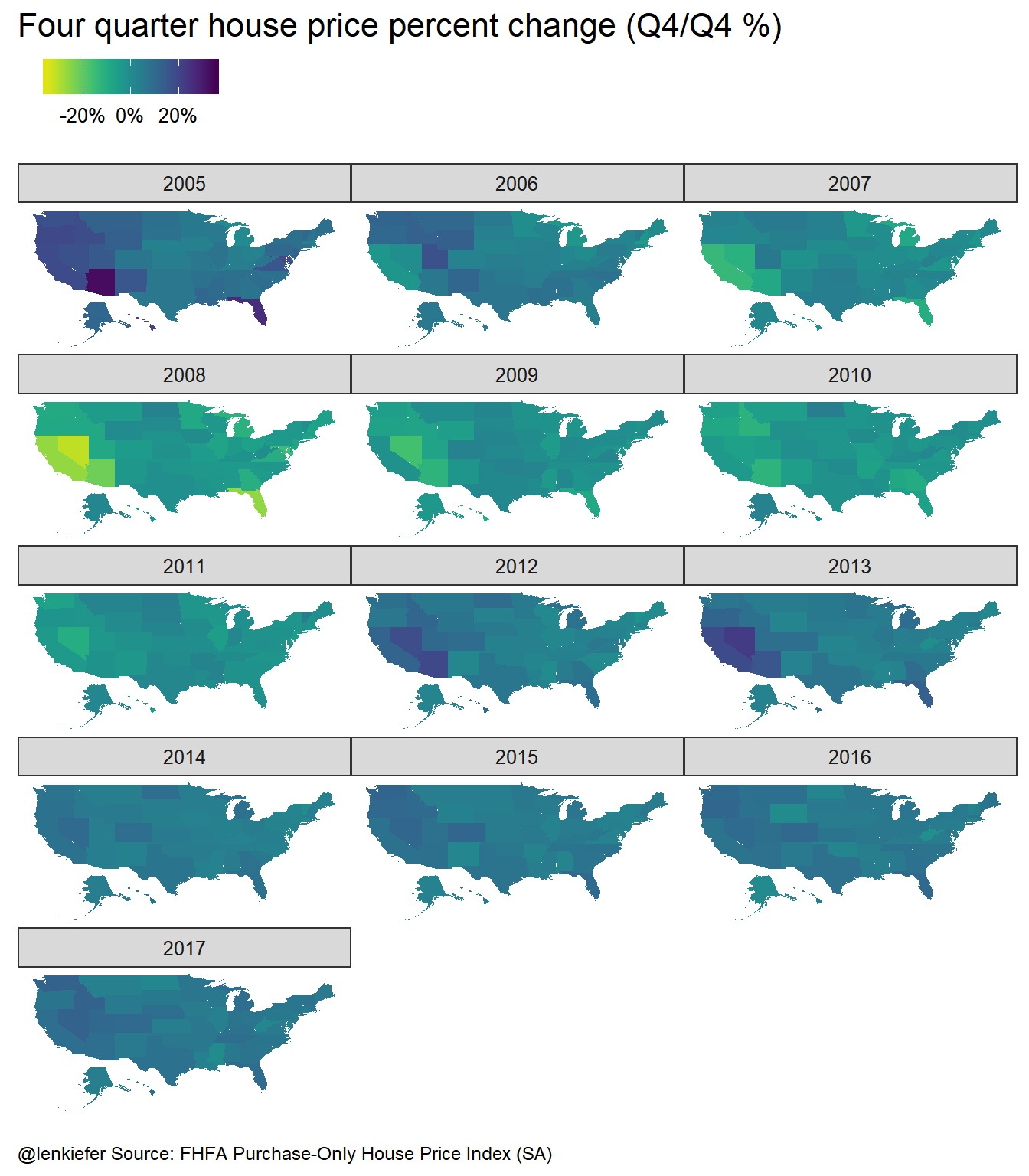
This map seems to do okay on the squint test. The extreme declines of 2008 and 2009 are clearly seen in the maps. But let’s use the pixelation trick to generate a pixelated version:
ggplot(filter(smap2,qtr==4 & yr>=2005),
             aes(round(long/3,0)*3,round(lat/3,0)*3, group=group, fill = hpa12)) +
      geom_polygon()+
      theme_map( base_size = 12) +facet_wrap(~yr,ncol=3)+
  theme(plot.title=element_text( size = 16, margin=margin(b=10))) +
  theme(plot.subtitle=element_text(size = 14, margin=margin(b=-20))) +
  theme(plot.caption=element_text(size = 9, margin=margin(t=-15))) +
  labs(title="",subtitle="" ) +
  scale_fill_viridis(name = "", discrete=F,option="D",end=0.95,
                     direction=-1,limits=c(-0.35,0.35),label=percent)+
  theme(legend.position = "top",
        plot.caption=element_text(hjust=0,                                                                  vjust=1,margin=margin(t=10)))+
  labs(title=paste0("Four quarter house price percent change (Q4/Q4 %)"),
       caption="@lenkiefer Source: FHFA Purchase-Only House Price Index (SA)")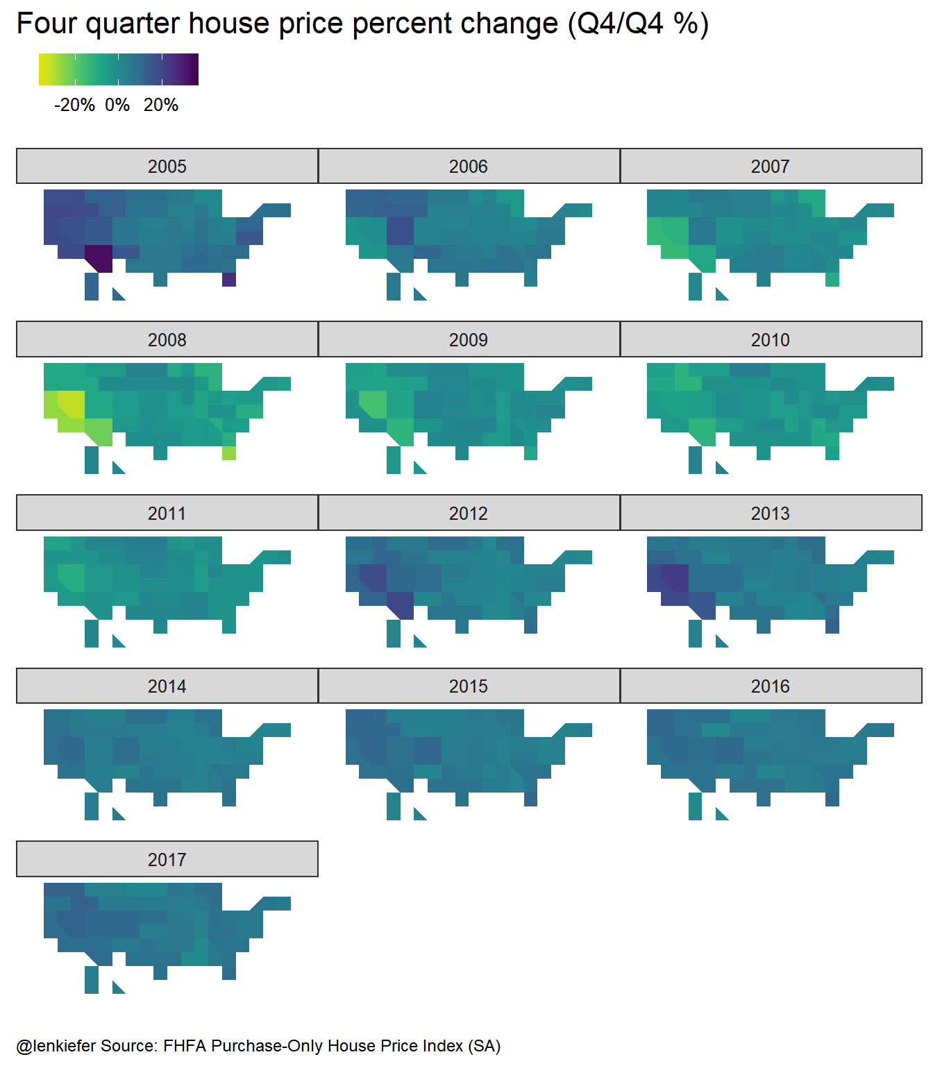
Okay, so even with our simulated squint, the key patterns still seem visible.