class: center, middle, inverse, title-slide # Forecasting Recessions with Dynamic Logistic Regression and Dynamic Model Averaging ### Len Kiefer ### 2017/10/31 --- # Overview * Motivation * Statistical model(s) * Empirical Excercise * Discussion --- class: inverse, center, middle # Motivation ## Uncertainty and Ambiguity --- class: left, top ### Statistical model(s) Application of *Dynamic Logistic Regression and Dynamic Model Averaging for Binary Classification* [LINK](https://www.ncbi.nlm.nih.gov/pubmed/21838812) We want to predict a binary outcome: `$$y_{t} \in (0,1)$$` where 1 (0) indicates recession (no recession). `$$y_{t}|L_{t}=k\sim Bernoulli(p_{t}^{(k)})$$` `$$Logit(p_{t}^{(k)}) = x^{(k)'}_{t-h}\theta^{(k)}_{t-h}$$` with `\(k=1,2,\ldots,K\)` possible models. --- class: inverse, center, middle ### Each model just your standard S curve 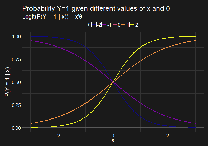<!-- --> --- class: left, top ### Suppose k=2 `$$Logit(P(y_{t}=1|x,L=1))= x_{1t}^{'}\theta_{t-h}^{(1)}$$` and `$$Logit(P(y_{t}=1|x,L=2))=x_{2t}^{'}\theta_{t-h}^{(2)}$$`. Parameters might be unstable and drift over time. A simple model of drift would be: `$$\theta_{t}^{(k)}=\theta_{t-1}^{(k)}+\delta^{(k)}_{t},\ \ \ \delta^{(k)}_{t} \sim N(0,\sigma^{2})$$` Suppose we have a way to estimate each model, how do we combine the results from `\(K\)` potential models? --- class: left, top ### Doing in the hard way Specify: `$$P(L_{t}=k|Y^{t-1}) = \sum_{\ell=1}^{K}p(L_{t-1}=\ell|Y^{t-1})p(L_{t}=k|L_{t-1}=\ell)$$` but `\(p(L_{t}=k|L_{t-1}=\ell)\)` requires a `\(K\times K\)` transition matrix. --- class: left, top ### Generally a hard problem to solve so <span style="color:#00b0f0";>forget about it</span> - Simplify via *forgetting factors* + See [this paper](https://www.ncbi.nlm.nih.gov/pmc/articles/PMC2895940/) *Online Prediction Under Model Uncertainty via Dynamic Model Averaging: Application to a Cold Rolling Mill* + See [this paper](https://www.ncbi.nlm.nih.gov/pubmed/21838812) *Dynamic Logistic Regression and Dynamic Model Averaging for Binary Classification* + See [this paper](http://onlinelibrary.wiley.com/doi/10.1111/j.1468-2354.2012.00704.x/pdf) *Forecasting Inflation Using Dynamic Model Averaging* + [R](https://www.r-project.org/) package [dma](https://CRAN.R-project.org/package=dma) --- class: left, to ### Forgetting instead of this: `$$p(L_{t}=k|L_{t-1}=\ell)$$` use: `$$P(L_{t}=k | Y^{t-1})= \frac{P(L_{t-1}=k | Y^{t-1})^{\alpha} }{\sum_{j=1}^{K}P(L_{t-1}=j | Y^{t-1})^{\alpha}}$$` Instead of specifying a full `\(K \times K\)` transition Matrix P for model probabilities, probabilities are updated using *forgetting*, parameterized by `\(0<\alpha\leq1\)`. The parameter `\(\alpha\)` determines how much weight is put on recent models. With `\(\alpha=1\)` there is no forgetting, but `\(\alpha<1\)` puts less weight on observations in the distant past. --- class: inverse, center, middle # Empirical example ### Forecasting recessions --- class: top, left ### Forecasting recessions 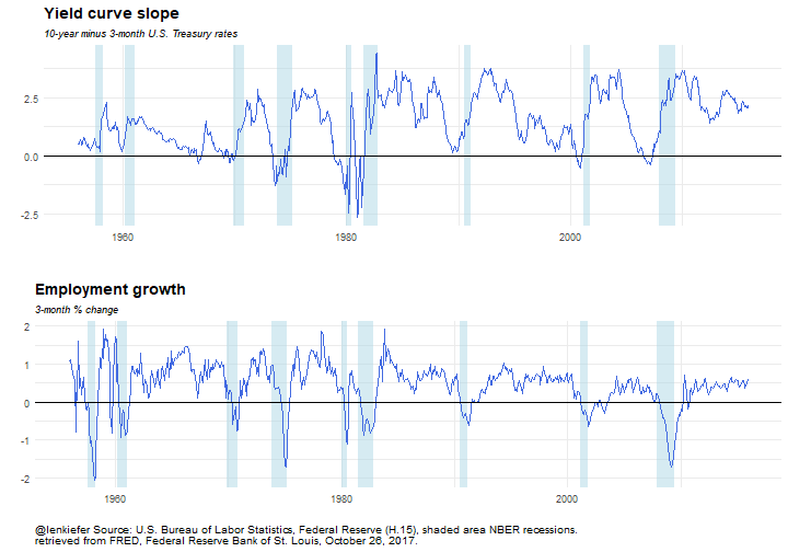<!-- --> --- class: top, left ### Static regression <table style="text-align:center"><caption><strong>Forecasting Recessions</strong></caption> <tr><td colspan="3" style="border-bottom: 1px solid black"></td></tr><tr><td style="text-align:left"></td><td colspan="2">Recession probability</td></tr> <tr><td></td><td colspan="2" style="border-bottom: 1px solid black"></td></tr> <tr><td style="text-align:left"></td><td>contemporaneous</td><td>forecast</td></tr> <tr><td style="text-align:left"></td><td>(h=0)</td><td>(h=12)</td></tr> <tr><td style="text-align:left"></td><td>(1)</td><td>(2)</td></tr> <tr><td colspan="3" style="border-bottom: 1px solid black"></td></tr><tr><td style="text-align:left">SLOPE</td><td>-0.964^***</td><td>-1.350^***</td></tr> <tr><td style="text-align:left"></td><td>(0.155)</td><td>(0.143)</td></tr> <tr><td style="text-align:left"></td><td></td><td></td></tr> <tr><td style="text-align:left">PAYEMS</td><td>-5.370^***</td><td>-0.046</td></tr> <tr><td style="text-align:left"></td><td>(0.529)</td><td>(0.231)</td></tr> <tr><td style="text-align:left"></td><td></td><td></td></tr> <tr><td style="text-align:left">Constant</td><td>-0.072</td><td>-0.528^***</td></tr> <tr><td style="text-align:left"></td><td>(0.230)</td><td>(0.196)</td></tr> <tr><td style="text-align:left"></td><td></td><td></td></tr> <tr><td colspan="3" style="border-bottom: 1px solid black"></td></tr><tr><td style="text-align:left">Observations</td><td>720</td><td>720</td></tr> <tr><td colspan="3" style="border-bottom: 1px solid black"></td></tr><tr><td style="text-align:left"><em>Note:</em></td><td colspan="2" style="text-align:left">^*p<0.1; ^**p<0.05; ^***p<0.01</td></tr> <tr><td style="text-align:left"></td><td colspan="2" style="text-align:left">Dependent variable is a 0/1 recession indicator. PAYEMS is 3-month % change in payroll employment. SLOPE is the slope of the U.S. Treasury yield curve (10-year minus 3-month Treasury rates).</td></tr> </table> --- class: left, middle ### Dynamic regressions (h=0) 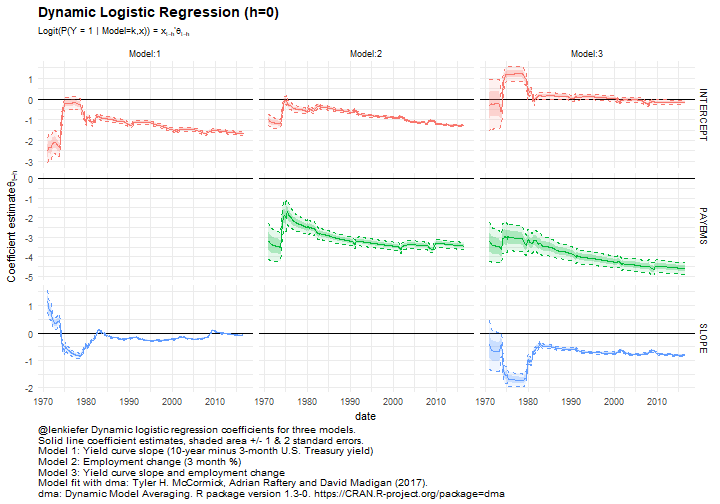<!-- --> --- class: top, left ### Model probabilties (h=0) 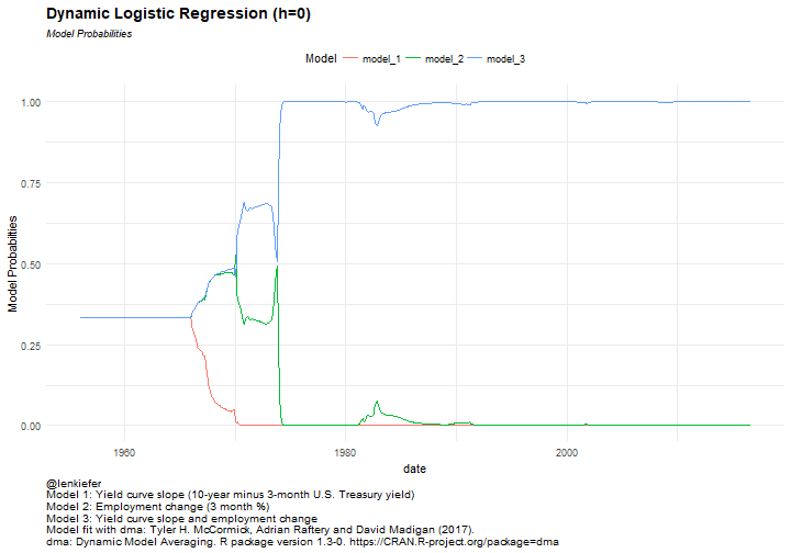<!-- --> --- class: left, middle ### Dynamic regressions (h=12) <!-- --> --- class: top, left ### Model probabilities (h=12) <!-- --> --- class: top, left ### Combining forecasts <!-- --> --- class: inverse, middle,center # Discussion ###<span style="color:#00b0f0";>How could we use this?</span>